Gene Finding
Gene Finding. Finding Genes. Prokaryotes Genome under 10Mb >85% of sequence codes for proteins Eukaryotes Large Genomes (up to 10Gb) 1-3% coding for vertebrates. Introns. Humans 95% of genes have introns 10% of genes have more than 20 introns Some have more than 60

Gene Finding
E N D
Presentation Transcript
Finding Genes • Prokaryotes • Genome under 10Mb • >85% of sequence codes for proteins • Eukaryotes • Large Genomes (up to 10Gb) • 1-3% coding for vertebrates
Introns • Humans • 95% of genes have introns • 10% of genes have more than 20 introns • Some have more than 60 • Largest Gene (Duchenne muscular dystrophy locus) spans >2Mb (more than a prokaryote) • Average exon = 150b • Introns can interrupt Open Reading Frame at any position, even within a codon • ORF finding is not sufficient for Eukaryotic genomes
Open Reading Frames in Bacteria • Without introns, look for long open reading frame (start codon ATG, … , stop codon TAA, TAG, TGA) • Short genes are missed (<300 nucleotides) • Shadow genes (overlapping open reading frames on opposite DNA strands) are hard to detect • Some genes start with UUG, AUA, UUA and CUG for start codon • Some genes use TGA to create selenocysteine and it is not a stop codon
Eukaryotes • Maps are used as scaffolding during sequencing • Recombination is used to predict the distance genes are from each other (the further apart two loci are on the chromosome, the more likely they are to be separated by recombination during meiosis) • Pedigree analysis
Gene Finding in Eukaryotes • Look for strongly conserved regions • RNA blots - map expressed RNA to DNA • Identification of CPG islands • Short stretches of CG rich DNA are associated with the promoters of vertebrate genes • Exon Trapping - put questionable clone between two exons that are expressed. If there is a gene, it will be spliced into the mature transcript
Computational methods • Signals - TATA box and other sequences • TATA box is found 30bp upstream from about 70% of the genes • Content - Coding DNA and non-coding DNA differ in terms of Hexamer frequency (frequency with which specific 6 nucleotide strings are used) • Some organisms prefer different codons for the same amino acid • Homology - blast for sequence in other organisms
Genome Browser • http://genome.ucsc.edu/ • Tables • Genome browser
Non-coding RNA genes • Ribosomal rRNA, transfer tRNA can be recognized by stochastic context-free grammars • Detection is still an open problem
Hidden Markov Models (HMMs) • Provide a probabilistic view of a process that we don’t fully understand • The model can be trained with data we don’t understand to learn patterns • You get to implement one for the first lab!!
State Transitions • Markov Model Example. • -x= States of the Markov model • - a = Transition probabilities • - b = Output probabilities • - y = Observable outputs • How does this differ from a Finite State machine? • Why is it a Markov process?
Example • Distant friend that you talk to daily about his activities (walk, shop, clean) • You believe that the weather is a discrete Markov chain (no memory) with two states (rainy, sunny), but you cant observe them directly. You know the average weather patterns
Formal Description states = ('Rainy', 'Sunny') observations = ('walk', 'shop', 'clean') start_probability = {'Rainy': 0.6, 'Sunny': 0.4} transition_probability = { 'Rainy' : {'Rainy': 0.7, 'Sunny': 0.3}, 'Sunny' : {'Rainy': 0.4, 'Sunny': 0.6}, } emission_probability = { 'Rainy' : {'walk': 0.1, 'shop': 0.4, 'clean': 0.5}, 'Sunny' : {'walk': 0.6, 'shop': 0.3, 'clean': 0.1}, }
Observations • Given (walk, shop, clean) • What is the probability of this sequence of observations? (is he really still at home, or did he skip the country) • What was the most likely sequence of rainy/sunny days?
Matrix Sunny, Rainy, Rainy = (.4*.6)(.4*.4)(.7*.5)
The CpG island problem • Methylation in human genome • “CG” -> “TG” happens in most places except “start regions” of genes and within genes • CpG islands = 100-1,000 bases before a gene starts • Question • Given a long sequence, how would we find the CpG islands in it?
How can we identify a CpG island in a long sequence? Idea 1: Test each window of a fixed number of nucleitides Idea2: Classify the whole sequence Class label S1: OOOO………….……O Class label S2: OOOO…………. OCC … Class label Si: OOOO…OCC..CO…O … Class label SN: CCCC……………….CC S*=argmaxS P(S|X) = argmaxS P(S,X) S*=OOOO…OCC..CO…O CpG Hidden Markov Model X=ATTGATGCAAAAGGGGGATCGGGCGATATAAAATTTG Other CpG Island Other
B I A simple HMM 0.7 Parameters Initial state prob: p(B)= 0.5; p(I)=0.5 State transition prob: p(BB)=0.7 p(BI)=0.3 p(IB)=0.5 p(II)=0.5 Output prob: P(a|B) = 0.25, … p(c|B)=0.10 … P(c|I) = 0.25 … 0.5 0.5 P(B)=0.5 P(I)=0.5 0.3 P(x|B) P(x|I) 0.5 0.5 P(x|HCpG)=p(x|I) P(a|I)=0.25 P(t|I)=0.25 P(c|I)=0.25 P(g|I)=0.25 P(x|HOther)=p(x|B) P(a|B)=0.25 P(t|B)=0.40 P(c|B)=0.10 P(g|B)=0.25
A General Definition of HMM Initial state probability: N states State transition probability: M symbols Output probability:
B I How to “Generate” a Sequence? P(x|B) P(x|I) 0.7 0.5 P(a|B)=0.25 P(t|B)=0.40 P(c|B)=0.10 P(g|B)=0.25 P(a|I)=0.25 P(t|I)=0.25 P(c|I)=0.25 P(g|I)=0.25 0.3 model 0.5 P(B)=0.5 P(I)=0.5 a c g t t … Sequence B I I I B B I B states I I I B B I I B … … Given a model, follow a path to generate the observations.
B I How to “Generate” a Sequence? P(x|B) P(x|I) 0.7 0.5 P(a|B)=0.25 P(t|B)=0.40 P(c|B)=0.10 P(g|B)=0.25 P(a|I)=0.25 P(t|I)=0.25 P(c|I)=0.25 P(g|I)=0.25 0.3 model 0.5 P(B)=0.5 P(I)=0.5 a c g t t … Sequence 0.3 0.5 0.5 0.5 B I I I B 0.5 0.25 0.25 0.25 0.25 0.4 t a c g t P(“BIIIB”, “acgtt”)=p(B)p(a|B) p(I|B)p(c|I) p(I|I)p(g|I) p(I|I)p(t|I) p(B|I)p(t|B)
HMM as a Probabilistic Model Time/Index: t1 t2 t3 t4 … Data: o1 o2 o3 o4 … Sequential data Random variables/ process Observation variable: O1 O2 O3 O4 … Hidden state variable: S1 S2 S3 S4 … State transition prob: Probability of observations with known state transitions: Output prob. Joint probability (complete likelihood): Init state distr. Probability of observations (incomplete likelihood): State trans. prob.