Graphs
Graphs. Graphs (part1). Basic concepts Graph representation Graph Searching Breadth-First Search Depth-First Search. Graphs. A graph G = (V, E) V = set of vertices E = set of edges = subset of V V |E| <= |V| 2. Directed/undirected graphs. In an undirected graph:

Graphs
E N D
Presentation Transcript
Graphs (part1) • Basic concepts • Graph representation • Graph Searching • Breadth-First Search • Depth-First Search
Graphs • A graph G = (V, E) • V = set of vertices • E = set of edges = subset of V V • |E| <= |V|2
Directed/undirected graphs • In an undirected graph: • Edge (u,v) E implies that also edge (v,u) E • Example: road networks between cities • In a directedgraph: • Edge (u,v) E does notimply edge (v,u) E • Example: street networks in downtown
Directed/undirected graphs • Self-loop edges are possible only in directed graphs Undirected graph Directed graph [CLRS] Fig 22.1, 22.2
Degree of a vertex • Degree of a vertex v: • The number of edges adjacenct to v • For directed graphs: in-degree and out-degree In-degree=2 Out-degre=1 degree=3
Weighted/unweighted graphs • In a weighted graph, each edge has an associated weight (numerical value)
Connected/disconnected graphs • An undirected graph is a connected graph if there is a path between any two vertexes • A directed graph is strongly connectedif there is a directed path between any two vertices
Dense/sparse graphs • Graphs are densewhen the number of edges is close to the maximum possible, |V|2 • Graphs are sparsewhen the number of edges is small (no clear threshold) • If you know you are dealing with dense or sparse graphs, different data structures are recommended for representing graphs • Adjacency matrix • Adjacency list
Representing Graphs – Adjacency Matrix • Assume vertexes are numbered V = {1, 2, …, n} • An adjacency matrixrepresents the graph as a n x n matrix A: • A[i, j] = 1 if edge (i, j) E = 0 if edge (i, j) E • For weighted graph • A[i, j] = wij if edge (i, j) E = 0 if edge (i, j) E • For undirected graph • Matrix is symmetric: A[i, j] = A[j, i]
Graphs: Adjacency Matrix • Example – Undirected graph:
Graphs: Adjacency Matrix • Example – Directed Unweighted Graph:
Graphs: Adjacency Matrix • Time to answer if there is an edge between vertex u and v: Θ(1) • Memory required: Θ(n2) regardless of |E| • Usually too much storage for large graphs • But can be very efficient for small graphs
Graphs: Adjacency List • Adjacency list: for each vertex v V, store a list of vertices adjacent to v • Weighted graph: for each vertex u adj[v], store also weight(v,u)
Graph representations • Adjacency list
Graph representations • Undirected graph
Graphs: Adjacency List • How much memory is required? • For directed graphs • |adj[v]| = out-degree(v) • Total number of items in adjacency lists is out-degree(v) = |E| • For undirected graphs • |adj[v]| = degree(v) • Number of items in adjacency lists is degree(v) = 2 |E| • Adjacency lists needs (V+E) memory space • Time needed to test if edge (u, v) E is O(E)
Graph Searching • Given: a graph G = (V, E), directed or undirected • Goal: methodically explore every vertex (and every edge) • Side-effect: build the subgraph resulting from the trace of this exploration • Different methods of exploration => • Different order of vertex discovery • Different shape of the exploration trace subgraph (which can be a spanning tree of the graph) • Methods of exploration: • Breadth-First Search • Depth-First Search
Breadth-First Search • Explore a graph by following rules: • Pick a source vertex to be the root • Expand frontierof explored vertices across the breadthof the frontier
Breadth-First Search • Associate vertex “colors” to guide the algorithm • White vertices have not been discovered • All vertices start out white • Grey vertices are discovered but not fully explored • They may be adjacent to white vertices • Black vertices are discovered and fully explored • They are adjacent only to black and gray vertices • Explore vertices by scanning adjacency list of grey vertices
Breadth-First Search • Every vertex v will get following attributes: • v.color: (white, grey, black) – represents its exploration status • v.pi represents the “parent” node of v (v has ben reached as a result of exploring adjacencies of pi) • v.d represents the distance (number of edges) from the initial vertex (the root of the BFS)
s=initial vertex (root) Mark all vertexes except the root as WHITE (not yet discovered) Mark root as GREY (start exploration) Use a Queue to store the exploration frontier Push s in Queue While there are nodes in the frontier (Queue) Pop a node u from Queue Discover all nodes v adjacent to u Mark u as fully explored
Example – Applying BFS r s t u v w x y
Example r s t u ∞ 0 ∞ ∞ ∞ ∞ ∞ ∞ v w x y Q s
Example r s t u 1 0 ∞ ∞ ∞ 1 ∞ ∞ v w x y Q w r
Example r s t u 1 0 2 ∞ ∞ 1 2 ∞ v w x y Q r t x
Example r s t u 1 0 2 ∞ 2 1 2 ∞ v w x y Q t x v
Example r s t u 1 0 2 3 2 1 2 ∞ v w x y Q x v u
Example r s t u 1 0 2 3 2 1 22 3 v w x y Q v u y
Example r s t u 1 0 2 3 2 1 22 3 v w x y Q u y
Example r s t u 1 0 2 3 2 1 22 3 v w x y Q y
Example r s t u 1 0 2 3 2 1 22 3 v w x y Q
Θ(V) Θ(E) Analysis Θ(V+E)
Analysis of BFS • If the graph is implemented using adjacency structures: • The adjacency list of each vertex is scanned only when the vertex is dequeued => every vertex is dequeued only once => the sum of the lengths of all adjacency lists is Θ(E) • The total time for BFS is O(V+E) • What if the graph is implemented using adjacency matrix ?
Shortest paths • In an unweighted graph, the shortest-path distance δ(s,v) from s to v is the minimum number of edges in any path from s to v. If there is no path from s to v, then δ(s,v)=∞
Properties of BFS • If G is a connected graph, then after BFS all its vertices will be BLACK. • For every vertex v, v.d is equal with the shortest path from s to v δ(s,v) • Proofs !
BFS trees • The procedure BFS builds a predecessor subgraph Gπ as it searches the graph G • The predecessor subgraph Gπ is a breadth-first tree if Vπ consists of the vertices reachable from s and, for all v in Vπ, the subgraph Gπ contains a unique simple path from s to v that is also a shortest path from s to v in G. • A breadth-first tree is indeed a tree, since it is connected and the number of its edges is with 1 smaller than the number of vertices.
Print shortest path from s to v • Assuming that BFS has already computed a breadth-first tree with the root s:
BFS Questions • What happens with BFS if G is not connected ? • Is it necessary to color nodes in BFS using 3 different colors ?
Depth-First Search • Depth-first search is another strategy for exploring a graph • Explore “deeper” in the graph whenever possible • Edges are explored out of the most recently discovered vertex v that still has unexplored edges • When all of v’s edges have been explored, backtrack to the vertex from which v was discovered
Depth-First Search • Vertices initially colored white • Then colored gray when discovered • Then black when their exploration is finished
Depth-First Search • Every vertex v will get following attributes: • v.color: (white, grey, black) – represents its exploration status • v.pi represents the “parent” node of v (v has ben reached as a result of exploring adjacencies of pi) • v.d represents the time when the node is discovered • v.f represents the time when the exploration is finished
Example – Applying DFS u v w x y z
Example – Applying DFS u v w 1/ x y z
Example – Applying DFS u v w 1/ 2/ x y z
Example – Applying DFS u v w 1/ 2/ 3/ x y z
Example – Applying DFS u v w 1/ 2/ 4/ 3/ x y z
Example – Applying DFS u v w 1/ 2/ 4/5 3/ x y z
Example – Applying DFS u v w 1/ 2/ 4/5 3/6 x y z