Download

1 / 27
290 likes | 614 Views
Earthwork. Cross Section and Borrow Pit Methods. This lecture covers: Readings: 26-1 to 26-6, 26-8 to 26-10. Figures: 26-1 to 26-4, 26-6, and 26-7 Plate B-5 page 893, and B-2 page 890 Examples:26-1 and 26-3. Volumes. Usage: Quantities of earthwork and concrete

E N D
Earthwork Cross Section and Borrow Pit Methods
This lecture covers: • Readings: 26-1 to 26-6, 26-8 to 26-10. • Figures: 26-1 to 26-4, 26-6, and 26-7 • Plate B-5 page 893, and B-2 page 890 • Examples:26-1 and 26-3
Volumes • Usage: • Quantities of earthwork and concrete • Capacities of some structures: tanks,.. • Quantities of water discharged by streams per unit time • Units: • 1 yd3 = 27ft3 • 1 m3 = 35.315ft3 • Acre-foot: volume of an acre of 1 foot depth
The Cross Section Method • More accurate than a single profile along the centerline. • Done by measuring cross sections (profiles) at a right angles to the centerline, usually at intervals of 50, or 100 ft. • Readings at each cross section are taken at the centerline and at critical points perpendicular to the centerline. • Cross sections are drawn and design templates are superimposed, the difference in area is the area of cut or fill at that section (end area).
End areas can be cut, fill, or transition (both). • Use the areas to compute volumes, knowing the distance between the sections. • The whole work can be done with photogrammetry and a computer software.
Data Recording • Plate B-5 • Left page looks like Profile leveling, no intermediate points • right page: in front of each station, a group of fractions that describe the point location, reading, and elevation, in the form: 99.2 7.4 52 Elevation rod reading distance from CL
End Area Computation • Simple cases: formulae in fig 26-2, and fig26-4 • End areas by coordinates: we will learn it through (traversing)
End Area Computation • Simple cases: formulae in fig 27-2, and fig 27-4
compute individual areas and add them up. After computing the elevation at critical points, form a table:(mistakes!) station H L C D E R G 24+00 0 C12.5 C15.8 C18.0 C10.1 C12.2 0 15 15 33.8 20 0 33.3 15 Compute the areas and add them up.
Volume Computation • Done after computing the end areas, identify which is cut and which is fill. Two main methods: • Average End Area: Multiply the average area of the two sections by the distance between them. See next slide • Ve = A1+ A2 * L yd3 2 27
Prismoidal Formula • What is a prismoid? A solid with parallel ends joined by a plane or continuously wrapped surfaces • Fits most earthwork problems • VP = L(A1+4AM+A2) yd3 • 6*27 • Where AM is the area of computed section midway between stations. • Prismodial Formula is more accurate, The difference is called CP: Prismoidal correction
Volume Computation • Compute end areas at stations, fill the first three columns in table 26-3. • Compute the cut and fill volumes, one of the formulae. • Multiply the fill volumes by an expansion factor. • Compute the amount of soil to be borrowed or transferred out of the site, which is the difference between the cut and the fill.
Borrow-Pit Method • Not suitable for linear features, very useful for construction sites. • The site is divided into equal squares of sides 20,50, or a 100 ft. Elevations are then measured at the corners of the grid, which are given titles that correspond to the coordinates of the corner in the grid, ex: 3-D, 4-A,.. • V = (hijn) A yd3 4*27 • The idea is to multiply each height by the number of complete squares it is common to. ( )
The volume of any square, or part of a square is equal to the average height(elevation difference) at the corners, times the area. To compute the volume: 1- draw a line between the cut and the fill areas 2- compute the total volume of all the complete cut squares, do the same for the fill, use the previous formula 3- Compute the incomplete squares separately and add them to the squares. 4- Compute the difference between the cut and the fill., pay attention to the expansion factor.
Site 1 Site 3 Site 2
Assumed 36 for piles 200 ft
C D B A