Week 7 Lecture 1+2
460 likes | 489 Views
Week 7 Lecture 1+2. Digital Communications System Architecture + Signals basics. Old Communication : Analog. Next Slide. Next Slide. Today: we use “Digital”. Block Diagram on Digital Communication Systems. Review: Why Digital Comm ?. Continuous Info. Source. Quantizer. Source Encoder.

Week 7 Lecture 1+2
E N D
Presentation Transcript
Week 7 Lecture 1+2 Digital Communications System Architecture + Signals basics
Old Communication : Analog Next Slide
Today: we use “Digital” Block Diagram on Digital Communication Systems
Continuous Info. Source Quantizer Source Encoder Sampler • The points may be considered as the input of a Digital Communication System where messages consist of sequences of "symbols" selected from an alphabet e.g. levels of a quantizer or telegraph letters, numbers and punctuations. • • The objective of a Source Encoder (or data compressor) is to represent the message-symbols arriving at point A2 by as few digits as possible. Thus, each level (symbol) at point is A2 mapped, by the Source Encoder, to a unique codeword of 1s and 0s and, at point B ,we get a sequence of binary digits.
There are two ways to reduce the channel noise/interference effects: 1. to introduce deliberately some redundancy in the sequence at point B and this is what a Discrete Channel Encoder does. This redundancy aids the receiver in decoding the desired sequence by detecting and many times correcting errors introduced by the channel; 2. to increase Transmitter's power - point T often very expensive therefore better to trade transmitter's power for channel bandwidth.
Digital Modulation Interleaver Discrete Channel Encoder Channel Encoder
De-Modulator DeInterleaver Channel Decoder
Receiver Source Decoder The source decoder processes the sequence received from the output of the channel decoder and, from the knowledge of the source encoding method used, attempts to reconstruct the signal of the information source.
A SIMPLIFIED BLOCK STRUCTURE (Digital source) Note: For Digital source -- Quality is measured as the Bit Error Rate (BER)
An Internet System (Digital source) based on Cellular Network in the core
Digital Transmission of Analogue Signals (voice) Not BER (like in Digital Source case, previous case)
It is clear from the previous discussion that signals (representing bits) propagate through the networks. Therefore the following sections are concerned with the main properties and parameters of communication signals.
Communication Signals Frequency Domain (Spectrum): very important in Communications
Classification of Signals according to their description
Classification of Signals: according to their periodicity
WOODWARD's Notation • The evaluation of FT, that is • involves integrating the product of a function and a complex exponential - which can be difficult; so tables of useful transformations are frequently used (next 2 slides). • However, the use of tables is greatly simplified by employing Woodward's notation for certain commonly occurring situations. • main advantage of using Woodward's notation: allows periodic time/frequency functions to be handled with FT rather than Fourier Series
Multiplication (TD) Convolution (FD) In FD, it becomes Shift operations!
we can generate any desired "rect" function by scaling and shifting; see for instance the following table effects of temporal scaling:
Bandwidth of a signal Bandwidth: the range of the significant frequency components in a signal waveform Examples of message signals (baseband signals) and their bandwidth: • television signal bandwidth 5.5MHz • speech signal bandwidth 4KHz • audio signal bandwidth 8kHz to 20kHz Examples of transmitted signals (basepass signals) and their bandwidth: • to be discussed latter on •Note that there are various definitions of bandwidth, e.g. 3dB bandwidth, null-to-null bandwidth, Nyquist (minimum) bandwidth (next slide)
REDUNDANCY The degree of similarity in a signal is provided by its Redundancy autocorrelation function. For instance the autocorrelation function of a signal
SIMILARITY The degree of similarity between two signals is given by their cross-correlation function. For instance the cross-correlation function between two signals
On Comm Noise • Usually people assume: Additive White Gaussian Noise (AWGN)