Exploring Fractals and Root-Finding Algorithms in Engineering
Learn the application of fractals in engineering, including the New-Raphson root-finding algorithm. Understand fractal dimensions and examples of fractal use in medical analysis, materials testing, and image compression.


Exploring Fractals and Root-Finding Algorithms in Engineering
E N D
Presentation Transcript
Computation & Simulation Assignment One New-Raphson root-finding algorithm Group 5 Tutor: Dr. Conor Brennan
Occurrence & use of fractals in engineering What are fractals? “A fractal is an object or quantity that displays self-similarity, in a somewhat technical sense, on all scales. The object need not exhibit exactly the same structure at all scales, but the same "type" of structures must appear on all scales. A plot of the quantity on a log-log graph versus scale then gives a straight line, whose slope is said to be the fractal dimension. The prototypical example for a fractal is the length of a coastline measured with different length rulers. The shorter the ruler, the longer the length measured, a paradox known as the coastline paradox.” (http://mathworld.wolfram.com/Fractal.html) Fractal comparison Fractal geometry v classical geometry Fractal dimension : “related to how fast the estimated measurement of the object increases as the measurement device becomes smaller” The higher the FD the more rapidly the measurement increases and the more irregular the fractal is. Wegner, T and Tyler, B. 1993. Fractal Creations. Corte Madera: The Waite Group. P. 16 How often used in engineering? A search of the Inspec(EI Engineering Village) Compendex database for 1969-2009 using the term “Fractal” resulted in 28248 records being returned (12 March 2009).
Fractal Use Examples: Medical Analysis Recognition of breast tumours by extracting and classifying fractal dimension spectra from medical images (98.8% accuracy). George, Loay E., Sager, Kamal H. 2007. Breast cancer diagnosis using multi-fractal dimension spectra. IEEE International Conference on Signal Processing and Communications, ICSPC 2007. Available from Inspec(EI Engineering Village) database .http://ieeexplore.ieee.org/ielx5/4712636/4728221/04728388.pdf?tp= [Accessed 12 March 2009]. Materials Analysis Non destructive testing of wood using x-ray computed tomography (CT) scanning and fractal dimension calculation to detect wood defects. Li, Li ,Qi, Dawei. 2007. Detection of cracks in computer tomography images of logs based on fractal dimension. IEEE International Conference on Automation and Logistics, ICAL 2007. Available from Inspec (EI Engineering Village) database .http://ieeexplore.ieee.org/ielx5/4338502/4338503/04338952.pdf?tp= [Accessed 12 March 2009].
Fractal Use Examples (cont) Image Compression Like fractals, self-similarity in a range of images can be represented using simple equations rather than drawing the image. This allows savings in image transmission and storage resources. Wegner, T and Tyler, B. 1993. Fractal Creations. Corte Madera: The Waite Group.
Use of Newton-Raphson methods in engineering Frequency of usage A search of the Inspec(EI Engineering Village) database for 1969-2009 using the term “Newton Raphson” resulted in 9477 records being returned (16 March 2009). Control Engineering Only 4-5 iterations of N-R required to converge upon the required frequency for the purpose of auto-tuning a proportional-integra-derivative (PID) controller => improved speed compared to some commercial controllers. Besharati Rad, A., Wai Lun Lo, Tsang, K.M. 1997. Self-tuning PID controller using Newton-Raphson search method . Industrial Electronics, IEEE Transactions onVolume 44, Issue 5, Oct. 1997 Page(s):717 - 725 .http://ieeexplore.ieee.org/stamp/stamp.jsp?tp=&arnumber=633479&isnumber=13741 [Accessed 16 March 2009].
Use of N-R (cont) Medical Mechanical Test to simulate contact conditions in a total knee replacement which used a NewtonRaphson method to solve the highly nonlinear system of equations involved. Kennedy, Francis E., Van Gitters, Douglas W., Wongseedakaew, Khanittha, Mongkolwongrojn, Mongkol. 2006. Lubrication and wear of artificial knee joint materials in a rolling/sliding tribotester. Proceedings of STLE/ASME International Joint Tribology Conference, IJTC 2006. http://www.engineeringvillage2.org/controller/servlet/Controller?SEARCHID=95215b12001c9f7e0M3c20prod4data2&CID=quickSearchDetailedFormat&DOCINDEX=1&database=3&format=quickSearchDetailedFormat[Accessed 16 March 2009] General Engineering Use - Important Consideration Accurate and fast processing is best achieved with an optimised initial point. This paper proposes a means of identifying such a starting point stating that that log scale based on geometric mean is most profitable initial point . ChangsoonChoi, Jinyong Lee, Younglok Kim. 2006 Initial point optimization for square root approximation based on Newton-Raphson method. Journal of the Institute of Electronics Engineers of Korea Volume: 43-SD Issue: 3 Publication date: March 2006 Pages: 15-20 http://www.engineeringvillage2.org/controller/servlet/Controller?CID=quickSearchDetailedFormat&SEARCHID=95215b12001c9f7e0M329cprod4data2&DOCINDEX=1&database=3&format=quickSearchDetailedFormat[Accessed 16 March 2009]
Assignment issues • Unknown roots of a function • How many roots? • When to stop N-R iterations? • How to compare all root approximations with each other
Code Structure • Determine the number of roots • Set up the parameters (complex plane, steps, flags, etc.) • Generate points in the complex plane • Implement N-R to determine convergence value for each point • Determine the function roots and allocate a colour for each root • Compare the convergence value of each point with the roots and assign the appropriate colour • Display the result
Matlab code • Determine the number of roots • Use an algorithm that iteratively differentiates the function to zero. • Number of roots is: Iterations – 1 • Generate points in the complex plane • Nested FOR loops iterate through every point in successive rows of the plane generating an array of complex numbers • Implement N-R to determine convergence values • Choice: • If function can be differentiated easily => use in N-R algorithm • If not => use SECANT method (Numerical approximation of the differentiation) • Number of iterations: • Compare successive approximation until the difference becomes tiny up to: • A maximum number of iterations • Maintain a count of number of iterations taken
Matlab code • Determine the function roots and allocate each a colour • Matrix to hold all possible root values • As convergence value (root approximation) for each start point is determined, compare it to each value already in the root matrix • If at the end of the comparison with the previously determined roots, the difference is > than a threshold, => approximation must be a previously undetermined root and is added to the next slot in the root matrix which has not been finalised and is also allocated a colour code. • Compare the convergence value of each point with the roots and assign the appropriate colour • If the approximation is “the same” (i.e. < threshold) as one of the previously determined roots it is allocated the same colour code as that root • Display the result
Fractal Images Fractal images based on the roots F(z)=z^3-1 F(z)=z^3-2z-1 F(z)=z^8+15z^4-16
Advantages • Single loop => speed • Determines each start point on the plane • Applies N-R to each point to get convergence value (root approximation) • Determines which of these will be the actual roots • Compares all the other approximations to the actual roots • Allocates appropriate colour codes to the start points • Generality • Code can be applied to different functions
Matlab code for shading • Similarities and differences • Similarites • code structure is the same as previous • Differences • Different colormap • Different color values be given to the color matrix
Matlab code • Part one—values for colormap • color_type=[spring ;summer ;autumn ;winter ;bone ;pink ; hsv ;hot ;cool ; copper]; • Each word is a matrix(64*3 matrix)
Matlab code • Part two— Given different values to the color matrix • Previous code: • color(ct1,ct2)=c; • For last code, colour data only depend on each root. • Shading code: • color(ct1,ct2)=(k-1)*64+step_matrix(ct1,ct2); • The value of k is depended on each root as well • (k-1)*64 determine the basic color will be used • Step matrix is used to record how many times this particular point runs N-R to find his root. • Step matrix determine the shading
Matlab code • Part three— draw the figures • Previous code: • colormap (jet) • Colour map is made up by one 64*3 matrix • Shading code: • colormap (color_type) • Color map is made up by eight*64*3 matrix
Matlab code for R.R. • Similarities and differences • Similarites • code structure is the same as previous • Differences • Using N-R twice • First double ‘for' loop—calculating root for original function • Second double ‘for’ loop--Rotation
Matlab code • Second Double ‘for’ loop • Exp(j*alpha) is used to rotate the original root on the unit circuit • Using a matrix which is named as ‘new_root’ to store these new roots • Using these new roots to find the new function and new derivative function A ‘for’ loop is used to determine the function. • F(x_old): calculate the function value when x=x_old • F(x_old+h): calculate the function value when x=x_old+h • Using Euler’s series to find the approx. derivative function • Then as previous, obtain the colour value for each point and output it.
Matlab code--Movie • We can also make a movie by storing these rotating pictures • Using getframe and movie method to store the pictures and play it together. • And also we can play a music when the movie is running. • [y fs]=wavread(‘name’) • sound(y, fs)
Challenge Three—Zoom In • function f(z)=z^3-1
Assignment One --basic • close all • clear all • use_secant = 0; • % Given a function calculate the no. of roots it has • % by repeating differentiation until zero reached. • number_of_roots=-1; • syms x • fun = the_func(x); • dy=1; • while (dy~=0) • dy=diff(fun); • fun=dy; • number_of_roots=number_of_roots+1; • end • % Set up parameters of plane • real_lower=-2.0; • real_upper=2.0; • imag_lower=-2.0; • imag_upper=2.0;
threshold = 1e-14 ; • % No of intervals in Real & Imag axes • N= 200; • % Length of each interval • real_step=[real_upper-real_lower]/N; • imag_step=[imag_upper-imag_lower]/N; • % X_new is the root approx, initialised to 0 • x_new=0; • % Matrix container to store the actual roots • root= zeros (number_of_roots,1); • % Root matrix field incrementer • k=1; • % Only relevant if secant mode used (ie = 1) • h=0.1; • % Max no of N-R iterations • max=99; • % Double FOR loop to go through every starting point on plane • for (ct1=1:N) • for (ct2=1: N) • % Generating actual points and storing them in z matrix (of start • % points). • z(ct1,ct2) = real_lower + (ct2-0.5)*real_step +j*(imag_lower + (ct1-0.5)*imag_step); • % X_Old will be the previous estimation of the root • x_old=z(ct1,ct2);
% Next 3 lines are Flags • b=0; • m=0; • steps=0; • %While loop implements N-R • while (b==0) & (steps<max) • if( use_secant == 0 ) • d = the_func_deriv(x_old) ; • else • d = (the_func(x_old + h) - the_func(x_old))/h ; • end • % Apply N-R • x_new = x_old - the_func(x_old) /d ; • % Compare each successive N-R approximation and if< • % threshold => x_new is a root. Else N-R runs again • if (abs(x_new-x_old)<threshold) • % Comapare each x_new root approximation to the • % current root values already sored in the root • % matrix • for (p=1:number_of_roots) • % If its > threshold => not converging on same • % root for each root value in root array then go • % to line after FOR loop • if(abs(root(p,1)-x_new)>threshold) • m=m+1; • % If < threshold => converging on same root as • % already in root array => just give it the same • % colour code • else • c=p; • end • end
% This just adds root to root array and sets • % the colour code if the conditions above • % fulfilled • if (m==number_of_roots) • root(k,1)=x_new; • % Colour matrix for every point in complex • % plane • color(ct1,ct2)=k; • % Increment root matrix field to accept next • % root • k=k+1; • % Jump out of WHILE loop (N-R implementation) • b=1; • % Apply the same colour code as the root • % already in the root array • else • color(ct1,ct2)=c; • % Colour output shows no of iterations of N-R • % (shading) • % color(ct1,ct2)=steps; • b=1; • end • end • % Continuation of the N-R • x_old=x_new; • % Counting the N-R iterations • steps=steps+1; • end • end • end
% Drawing the figures • figure • % Surface view of the colour matrix • surf (color) • % View from above • view ([0 90]) • % Provides smoother contours • shading interp • % Preset Type of colour mapping • colormap (jet) • figure • surf (color) • view ([0 90]) • shading interp • colormap (hot) • colorbar