Quiz 7: MDPs

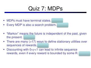
1. Quiz 7: MDPs • MDPs must have terminal states. False • Every MDP is also a search problem. False • “Markov” means the future is independent of the past, given the present. True • There are many (>17) ways to define stationary utilities over sequences of rewards. False • Discounting with 0<𝛾<1 can lead to infinite sequence rewards, even if every reward is bounded by some R. False

2. CS 511a: Artificial IntelligenceSpring 2013 Lecture 10: MEU / Markov Processes 02/18/2012 Robert Pless, Course adapted from one taught by Kilian Weinberge, with many slides over the course adapted from either Dan Klein, Stuart Russell or Andrew Moore

3. Announcements • Project 2 out • due Thursday, Feb 28, 11:59pm (1 minute grace period). • HW 1 out • due Friday, March 1, 5pm, accepted with no penalty (or charged late days) until Monday, March 4, 10am. • Midterm Wednesday March 6. • Class Wednesday? No! • Instead (if possible) attend talk by Alexis Battle, Friday, 11am, Lopata 101.

4. s a s, a s,a,s’ s’ Recap: Defining MDPs • Markov decision processes: • States S • Start state s0 • Actions A • Transitions P(s’|s,a) (or T(s,a,s’)) • Rewards R(s,a,s’) • Discount  • MDP quantities so far: • Policy = Choice of action for each state • Utility (or return) = sum of discounted rewards

5. Grid World • The agent lives in a grid • Walls block the agent’s path • The agent’s actions do not always go as planned: • 80% of the time, the action North takes the agent North (if there is no wall there) • 10% of the time, North takes the agent West; 10% East • If there is a wall in the direction the agent would have been taken, the agent stays put • Small (negative) “reward” each step • Big rewards come at the end • Goal: maximize sum of rewards*

6. Discounting • Typically discount rewards by  < 1 each time step • Sooner rewards have higher utility than later rewards • Also helps the algorithms converge

7. s a s, a R(s,a,s’) T(s,a,s’) s’ Optimal Utilities • Fundamental operation: compute the values (optimal expectimax utilities) of states s • Why? Optimal values define optimal policies! • Define the value of a state s: V*(s) = expected utility starting in s and acting optimally • Define the value of a q-state (s,a): Q*(s,a) = expected utility starting in s, taking action a and thereafter acting optimally • Define the optimal policy: *(s) = optimal action from state s V*(s) Q*(s,a) V*(s’) Quiz: Define V* in terms of Q* and vice versa!

8. s a s, a R(s,a,s’) T(s,a,s’) s’ The Bellman Equations • Definition of “optimal utility” leads to a simple one-step lookahead relationship amongst optimal utility values: Optimal rewards = maximize over first action and then follow optimal policy • Formally: V*(s) Q*(s,a) V*(s’)

9. s s, a R(s,a,s’) T(s,a,s’) s’ Solving MDPs • We want to find the optimal policy* • Proposal 1: modified expectimax search, starting from each state s: V*(s) a=*(s) Q*(s,a) V*(s’)

10. Why Not Search Trees? • Why not solve with expectimax? • Problems: • This tree is usually infinite (why?) • Same states appear over and over (why?) • We would search once per state (why?) • Idea: Value iteration • Compute optimal values for all states all at once using successive approximations • Will be a bottom-up dynamic program similar in cost to memoization • Do all planning offline, no replanning needed!

11. Value Estimates • Calculate estimates Vk*(s) • Not the optimal value of s! • The optimal value considering only next k time steps (k rewards) • As k  , it approaches the optimal value • Why: • If discounting, distant rewards become negligible • If terminal states reachable from everywhere, fraction of episodes not ending becomes negligible • Otherwise, can get infinite expected utility and then this approach actually won’t work

12. Value Iteration • Idea, Bellman equation is property of optimal valuations: • Start with V0*(s) = 0, which we know is right (why?) • Given Vi*, calculate the values for all states for depth i+1: • This is called a value update or Bellman update • Repeat until convergence • Theorem: will converge to unique optimal values • Basic idea: approximations get refined towards optimal values • Policy may converge long before values do

13. Example: =0.9, living reward=0, noise=0.2 Example: Bellman Updates max happens for a=right, other actions not shown =0.8·[0+0.9·1]+0.1·[0+0.9·0]+0.1[0+0.9·0]

14. Gridworld

15. Gridworld

16. Gridworld

17. Gridworld

18. Gridworld

19. Convergence* • Define the max-norm: • Theorem: For any two approximations U and V • I.e. any distinct approximations must get closer to each other, so, in particular, any approximation must get closer to the true U and value iteration converges to a unique, stable, optimal solution • Theorem: • I.e. once the change in our approximation is small, it must also be close to correct *

20. Example http://www.cs.ubc.ca/~poole/demos/mdp/vi.html

21. Policy Iteration Why do we compute V* or Q*, if all we care about is the best policy *?

22. s a s, a R(s,a,s’) T(s,a,s’) s’ Utilities for Fixed Policies • Another basic operation: compute the utility of a state s under a fix (general non-optimal) policy • Define the utility of a state s, under a fixed policy : V(s) = expected total discounted rewards (return) starting in s and following  • Recursive relation (one-step look-ahead / Bellman equation): V (s) Q*(s,a) a=(s)

23. Policy Evaluation • How do we calculate the V’s for a fixed policy? • Idea one: modify Bellman updates • Idea two: Optimal solution is stationary point (equality). Then it’s just a linear system, solve with Matlab (or whatever)

24. Policy Iteration • Policy evaluation: with fixed current policy , find values with simplified Bellman updates: • Iterate until values converge • Policy improvement: with fixed utilities, find the best action according to one-step look-ahead

25. Comparison • In value iteration: • Every pass (or “backup”) updates both utilities (explicitly, based on current utilities) and policy (possibly implicitly, based on current policy) • Policy might not change between updates (wastes computation)  • In policy iteration: • Several passes to update utilities with frozen policy • Occasional passes to update policies • Value update can be solved as linear system • Can be faster, if policy changes infequently • Hybrid approaches (asynchronous policy iteration): • Any sequences of partial updates to either policy entries or utilities will converge if every state is visited infinitely often

26. Asynchronous Value Iteration • In value iteration, we update every state in each iteration • Actually, any sequences of Bellman updates will converge if every state is visited infinitely often • In fact, we can update the policy as seldom or often as we like, and we will still converge • Idea: Update states whose value we expect to change: If is large then update predecessors of s

27. How does this all play out? • for blackjack