Download
1 / 23
230 likes | 300 Views
I was on the second day of a road trip when I decided to keep a record of how far I had traveled from home. The table below shows how many hours I drove that day and how far I was away from home. For example, after I had traveled a total of 3½ hours, I was 366 miles away from home.

E N D
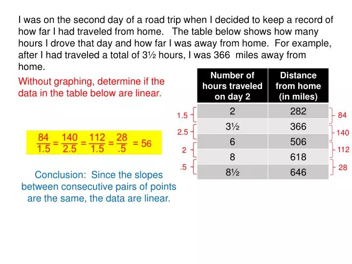
I was on the second day of a road trip when I decided to keep a record of how far I had traveled from home. The table below shows how many hours I drove that day and how far I was away from home. For example, after I had traveled a total of 3½ hours, I was 366 miles away from home. Without graphing, determine if the data in the table below are linear. 84 1.5 2.5 140 112 2 .5 28 Conclusion: Since the slopes between consecutive pairs of points are the same, the data are linear.
I was on the second day of a road trip when I decided to keep a record of how far I had traveled from home. The table below shows how many hours I drove that day and how far I was away from home. For example, after I had traveled a total of 3½ hours, I was 366 miles away from home. Without graphing, determine if the data in the table below are linear. • Exit Ticket • Find the linear model (equation) for the data. • Graph the data points and the model • on your calculator. Call your teacher • over to see your calculator screen. • How far was I from home at the start of the day? y = 56x + 170 x = number of hours y = distance in miles 170 miles
Answers to even-numbered HW problems Section 3.3 S-2 Since x-values are evenly spaced and y-values are not, the data are not linear. S-18 Calculator Graph Ex 2a) y = 1445x – 2,870,269 b) Graph c) The formula predicts a tuition of $34,181 for 2010. Ex 12b) The slope is -.09. It means number of graduates c) G = -.09y +181.48 where y = years and G = number of graduates in millions. d) G(1994) = 2.02 million 5 4 4 1445 1 The data are linear because all the dates increase by the same amount and all the tuitions increase by the same amount 1 1445 where x = years and y = tuition 1 1445 1 1445 decreased, on average, by .09 million (90,000) each year from 1985 to 1991. 2 .18 2 .18 2 .18 The data are linear because all the years increase by the same amount and the number of graduates decreases by the same amount The data are linear because the slope between each pair of points is the same (-.09)
1970 1975 1980 1985 1990 10 20 5 15 0 Years since 1970 The chart below represents the number of automobiles (in millions) produced worldwide in each of the years listed. Use the graphing calculator to make a scatter plot of the data using years since 1970.
1970 1975 1980 1985 1990 10 20 5 15 0 Years since 1970 The chart below represents the number of automobiles (in millions) produced worldwide in each of the years listed.
10 20 5 15 0 Years since 1970 Are the data approximately linear? Are the data linear? What linear function would be a good model for this data? y = .65x + 23.3 A = # of automobiles produced (in millions) t = number of years since 1970 A = .65t + 23.3
10 20 5 15 0 Years since 1970 The Regression Line (also called the least-squares fit line or the best fit line) for a set of data is a line that is, on average, closest to each data point. y = .65x + 23.3 A = # of automobiles produced (in millions) t = number of years since 1970 A = .65t + 23.3
1970 1975 1980 1985 1990 A = .65t + 23.3 10 20 5 15 0 Years since 1970 A = .648t + 22.78 A = # of automobiles produced (in millions) t = number of years since 1970 Regression equation: y = .648x + 22.78
1970 1975 1980 1985 1990 10 20 5 15 0 Years since 1970 A = .648t + 22.78 A = # of automobiles produced (in millions) t = number of years since 1970 Regression equation: y = .648x + 22.78 The slope (.648) means that automobile production increased, on average, by .648 million each year from 1970 to 1990. Question: Explain in practical terms the meaning of the slope of the regression line model.
1970 1975 1980 1985 1990 10 20 5 15 0 Years since 1970 A = .648t + 22.78 A = # of automobiles produced (in millions) t = number of years since 1970 Regression equation: y = .648x + 22.78 Question: What is the model’s estimate of automobile production in 1970? How far from the actual 1970 automobile production is the estimate?
1970 1975 1980 1985 1990 10 20 5 15 0 Years since 1970 A = .648t + 22.78 A = # of automobiles produced (in millions) t = number of years since 1970 Regression equation: y = .648x + 22.78 The model’s estimate for 1970 is 22.78 million cars produced. This differs from the actual figure by .52 million cars.
1970 1975 1980 1985 1990 10 20 5 15 0 Years since 1970 A = .648t + 22.78 A = # of automobiles produced (in millions) t = number of years since 1970 Regression equation: y = .648x + 22.78 Question: Use the regression equation to estimate automobile production in 2005.
1970 1975 1980 1985 1990 10 20 5 15 0 Years since 1970 A = .648t + 22.78 A = # of automobiles produced (in millions) t = number of years since 1970 Regression equation: y = .648x + 22.78 The model’s estimate for number of automobiles produced in 2005 is 45.46 million.
The model’s estimate for number of automobiles produced in 2005 is 45.46 million. Source: Worldwatch Institute http://www.worldwatch.org/node/4288
The model’s estimate for number of automobiles produced in 2005 is 45.46 million. “Global passenger car production grew in 2005 to 45.6 million units.” Source: Worldwatch Institute http://www.worldwatch.org/node/4288
Homework: Read Section 3.4 (through bottom of page 237) Page 278 # S-1, S-3, S-5 Pages 280 – 282 # 1, 2, 5, 9 * All graphs to be done on the calculator
The table below shows the population of the United States in millions. 0 10 20 30 Graph the data on a graphing calculator using years since 1960.
The table below shows the population of the United States in millions. 0 10 20 30 1. Find the equation of the regression line using years since 1960. 2. Identify the slope of the regression line and explain what it means in this setting. 3. Use the regression equation to estimate the U.S. population in the year 2000.
The table below shows the population of the United States in millions. 0 10 20 30 1. Find the equation of the regression line using years since 1960. 2. Identify the slope of the regression line and explain what it means in this setting. 3. Use the regression equation to estimate the U.S. population in the year 2000. y = 2.302x + 181.32 where x = years since 1960 and y = population in millions. The slope is 2.302. It means that the U.S. population increased, on average, by 2.302 million people per year from 1960 to 1990. Based on the model, the population of the U.S. in 2000 was 273.4 million.
The table below shows the population of the United States in millions. 0 10 20 30 Based on actual census figures, the actual U.S. population in 2000 was 281,421,906. Based on the model, the population of the U.S. in 2000 was 273.4 million.