Download
1 / 53
530 likes | 641 Views
Calibration, Imaging and Analysis of Data Cubes. Ylva Pihlström UNM. Outline. Why spectral line (multi-channel) observing? Not only for spectral lines, but there are many advantages for continuum experiments as well Calibration specifics Bandpass, flagging, continuum subtraction

E N D
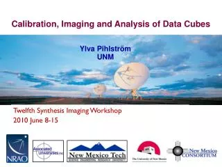
Calibration, Imaging and Analysis of Data Cubes Ylva Pihlström UNM
Twelfth Synthesis Imaging Workshop Outline • Why spectral line (multi-channel) observing? • Not only for spectral lines, but there are many advantages for continuum experiments as well • Calibration specifics • Bandpass, flagging, continuum subtraction • Imaging of spectral line data • Visualizing and analyzing cubes
Twelfth Synthesis Imaging Workshop Introduction Spectral line observers use many channels of width , over a total bandwidth . Why? • Science driven: science depends on frequency (spectroscopy) • Emission and absorption lines, and their Doppler shifts • Slope across continuum bandwidth • Technical reasons: science does not depend on frequency (pseudo-continuum)
Twelfth Synthesis Imaging Workshop Spectroscopy • Need high spectral resolution to resolve spectral features • Example: SiO emission from inner part of a protostellar jet imaged with the VLA. • High resolutions over large bandwidths are useful for e.g., Doppler shifts and line searches => many channels desirable! Chandler & Richer (2001)
Twelfth Synthesis Imaging Workshop Pseudo-continuum • Science does not depend on frequency, but using spectral line mode is favorable to correct for, at least some, frequency dependent issues: • Limitations of bandwidth smearing • Limitations of beam smearing • Problems due to atmospheric changes as a function of frequency • Problems due to signal transmission effects as a function of frequency • Using a spectral line mode also allows editing for unwanted, narrow-band interference.
Twelfth Synthesis Imaging Workshop 2 Instrument response: beam smearing • θPB = l/D • Band covers l1 -l2 θPB changes by l1/l2 • More important at longer wavelengths: • VLA 20cm: 1.03 • VLA 2cm: 1.003 • EVLA 20cm: 2.0 • EVLA 2cm: 1.5 • ALMA 1mm: 1.03
Twelfth Synthesis Imaging Workshop Instrument response: bandwidth smearing • Also called chromatic aberration • Fringe spacing = l/B • Band covers l1 -l2 • Fringe spacings change by l1/l2 • u,v samples smeared radially • More important in larger configurations, and for lower frequencies • Huge effects for EVLA u vs. v for VLA A-array, ratio 2.0 Pseudo-continuum uses smaller ranges to be averaged later.
Twelfth Synthesis Imaging Workshop Instrument frequency response • Responses of antenna receiver, feed IF transmission lines, electronics are a function of frequency. Tsys @ 7mm VLA • Phase slopes (delays) can be introduced by incorrect clocks or positions. VLBA
Twelfth Synthesis Imaging Workshop Atmosphere and source changes with frequency • The opacity, phase (delay) and Faraday rotation are functions of frequency • Generally only important over very wide bandwidths or near atmospheric lines • The source change with frequency too: • Spectral index, shape • Polarized emission; Faraday rotation 2 Chajnantor pwv = 1mm O2H2O VLA pwv = 4mm = depth of H2O if converted to liquid
Twelfth Synthesis Imaging Workshop Radio Frequency Interference (RFI) • Avoid known RFI if possible, e.g. by constraining your bandwidth • Use RFI plots posted online for EVLA & VLBA RFI at the EVLA 1-2 GHz
Twelfth Synthesis Imaging Workshop Example RFI at the VLBA
Twelfth Synthesis Imaging Workshop Spectral response • For spectroscopy in an XF correlator (EVLA) lags are introduced • The correlation function is measured for a large number of lags. • The FFT gives the spectrum. • We don't have infinitely large correlators and infinite amount of time, so we don't measure an infinite number of Fourier components. • A finite number or lags means a truncated lag spectrum, which corresponds to multiplying the true spectrum by a box function. • The spectral response is the FT of the box, which for an XF correlator is a sinc(x) function with nulls spaced by the channel separation: 22% sidelobes!
Twelfth Synthesis Imaging Workshop Spectral response: Gibb's ringing • Produces a "ringing" in frequency called the Gibbs phenomenon. • Occurs at sharp transitions: • Narrow banded spectral lines (masers, RFI) • Band edges • Baseband (zero frequency) "Ideal" spectrum Measured spectrum Amp Amp Frequency Frequency
Twelfth Synthesis Imaging Workshop Gibb's ringing: remedies • Increase the number of lags, or channels. • Oscillations reduce to ~2% at channel 20, so discard affected channels. • Works for band-edges, but not for spectral features. • Smooth the data in frequency (i.e., taper the lag spectrum) • Usually Hanning smoothing is applied, reducing sidelobes to <3%.
Twelfth Synthesis Imaging Workshop Calibration • Data editing and calibration is not fundamentally different from continuum observations, but a few additional items to consider: • Presence of RFI (data flagging) • Bandpass calibration • Doppler corrections • Correlator setup • Larger data sets
Twelfth Synthesis Imaging Workshop Editing spectral line data • Start with identifying problems affecting all channels, but using a frequency averaged 'channel 0' data set. • Has better signal-to-noise ratio (SNR) • Copy flag table to the line data • Continue with checking the line data for narrow-band RFI that may not show up in averaged data. • Channel by channel is very impractical, instead identify features by using cross- and total power spectra (POSSM)
Twelfth Synthesis Imaging Workshop Example POSSM scalar averaged spectra VLBA • Is it limited in time? Limited to specific telescopes? • Using VPLOT to plot the RFI affected channels as a function of time can be useful to identify bad time ranges and antennas. Scalar averaging helps to identify RFI features
Twelfth Synthesis Imaging Workshop Example SPFLG of one baseline • Flag based on the feature using SPFLG, EDITR, TVFLG, WIPER, also UVPLT, UVPRT, UVFLG. • Note: avoid excessive frequency dependent editing, since this introduces changes in the u,v - coverage across the band.
Twelfth Synthesis Imaging Workshop Why bandpass calibration? • Important to be able to detect and analyze spectral features: • Frequency dependent amplitude errors limit the ability of detecting weak emission and absorption lines. • Frequency dependent phase errors can lead to spatial offsets between spectral features, imitating Doppler motions. • Frequency dependent amplitude errors can imitate changes in line structures. • For pseudo-continuum, the dynamic range of final image is limited by the bandpass quality.
Twelfth Synthesis Imaging Workshop Example ideal and real bandpass Ideal Real • In the bandpass calibration we want to correct for the offset of the real bandpass from the ideal one (amp=1, phase=0). • The bandpass is the relative gain of an antenna/baseline as a function of frequency. Phase Amp
Twelfth Synthesis Imaging Workshop Bandpass calibration • We need the total response of the instrument to determine the true visibilities from the observed: • The bandpass shape is a function of frequency, and is mostly due to electronics of individual antennas. • Usually varies slowly with time, so we can break the complex gain Gij(t) into a fast varying frequency independent part, and a slowly varying frequency dependent part:
Twelfth Synthesis Imaging Workshop Bandpass calibration • G'i,j is calibrated as for continuum, for Bi,j we usually observe a bright continuum source • The frequency spectrum of visibilities for a flat-spectrum source should give a direct estimate of the bandpass for each baseline: • Requires a very high SNR • Instead we often solve for antenna based gains:
Twelfth Synthesis Imaging Workshop How bandpass calibration is performed • The most commonly used method is analogous to channel by channel self-calibration (AIPS task BPASS) • The calibrator data is divided by a source model or continuum, which removes atmospheric and source structure effects. • Most frequency dependence is antenna based, and the antenna-based gains bi(t,) are solved for as free parameters. • Less computationally expensive than baseline-based computed gains, and gives solutions for all antennas even if baselines are missing. • This requires a high SNR, so what is a good choice of a BP calibrator?
Twelfth Synthesis Imaging Workshop How to select a BP calibrator • Select a continuum source with: • High SNR in each channel • Intrinsically flat spectrum • No spectral lines • Not required to be a point source, but helpful since the SNR will be the same in the BP solution for all baselines • Also don't want it to be resolved out at long baselines Not good, line feature Too weak Good
Twelfth Synthesis Imaging Workshop How long to observe a bandpass calibrator • Applying the BP calibration means that every complex visibility spectrum will be divided by a complex bandpass, so noise from the bandpass will degrade all data. • Need to spend enough time on the BP calibrator so that SNRBPcal > SNRtarget. A good rule of thumb is to use SNRBPcal > 3SNRtarget which then results in an integration time: tBPcal = 9(Starget /SBPcal)2 ttarget • Observe several times in your experiment to account for slow time variations
Twelfth Synthesis Imaging Workshop Assessing quality of bandpass calibration Examples of good-quality bandpass solutions for 2 antennas: • Solutions should look comparable for all antennas. • Mean amplitude ~1 across useable portion of the band. • No sharp variations in amplitude and phase; variations are not dominated by noise. Phase Amp Phase Amp
Twelfth Synthesis Imaging Workshop Bad quality bandpass solutions • Amplitude has different normalization for different antennas • Noise levels are high, and are different for different antennas Phase Amp
Twelfth Synthesis Imaging Workshop Bandpass quality: apply to a continuum source • Before accepting the BP solutions, apply to a continuum source and use cross-correlation spectrum to check: • That phases are flat • That amplitudes are constant • That the noise is not increased by applying the BP Before bandpass calibration After bandpass calibration
Twelfth Synthesis Imaging Workshop Doppler tracking • Observing from the surface of the Earth, our velocity with respect to astronomical sources is not constant in time or direction. • Doppler tracking can be applied in real time to track a spectral line in a given reference frame, and for a given velocity definition: (approximations to relativistic formulas)
Twelfth Synthesis Imaging Workshop Rest frames Start with the topocentric frame, the successively transform to other frames. Transformations standardized by IAU.
Twelfth Synthesis Imaging Workshop Doppler tracking • Note that the bandpass shape is really a function of frequency, not velocity! • Applying Doppler tracking will introduce a time-dependent and position dependent frequency shift. • If you Doppler track your BP calibrator to the same velocity as your source, it will be observed at a different sky frequency! • If differences large, apply corrections during post-processing instead. • Given that wider bandwidths are now being used (EVLA, SMA, ALMA) online Doppler tracking may not be used in the future (tracking only correct for a single frequency).
Twelfth Synthesis Imaging Workshop Doppler corrections in post-processing • Calculate the sky frequency for, e.g., the center channel of your target source depending on RA, Dec, rest frequency, velocity frame and definition, and time of observations (EVLA has an online Dopset Tool) • Enter this information into CVEL which will perform necessary shifts. Amp Amp Channel Channel Before and after Doppler correction
Twelfth Synthesis Imaging Workshop Before imaging • We have edited the data, and performed band pass calibration. Also, we have done Doppler corrections if necessary. • Before imaging a few things can be done to improve the quality of your spectral line data • Image the continuum in the source, and perform a self-calibration. Apply to the line data: • Get good positions of line features relative to continuum • Can also use a bright spectral feature, like a maser • For line analysis we want to remove the continuum
Twelfth Synthesis Imaging Workshop Continuum subtraction • Spectral line data often contains continuum emission, either from the target or from nearby sources in the field of view. • This emission complicates the detection and analysis of line data Spectral line cube with two continuum sources (structure independent of frequency) and one spectral line source. Roelfsma 1989
Twelfth Synthesis Imaging Workshop Continuum subtraction: basic concept • Use channels with no line features to model the continuum • Subtract this continuum model from all channels
Twelfth Synthesis Imaging Workshop Why do continuum subtraction? • Spectral lines easier to see, especially weak ones in a varying continuum field. • Easier to compare the line emission between channels. • Deconvolution is non-linear: can give different results for different channels since u,v - coverage and noise differs • results usually better if line is deconvolved separately • If continuum sources exists far from the phase center, we don't need to deconvolve a large field of view to properly account for their sidelobes. To remove the continuum, different methods are available: visibility based, image based, or a combination thereof.
Twelfth Synthesis Imaging Workshop Visibility based continuum subtraction (UVLIN) • A low order polynomial is fit to a group of line free channels in each visibility spectrum, the polynomial is then subtracted from whole spectrum. • Advantages: • Fast, easy, robust • Corrects for spectral index slopes across spectrum • Can do flagging automatically (based on residuals on baselines) • Can produce a continuum data set • Restrictions: • Channels used in fitting must be line free (a visibility contains emission from all spatial scales) • Only works well over small field of view << s / tot
Twelfth Synthesis Imaging Workshop UVLIN restriction: small field of view • A consequence of the visibility of a source being a sinusoidal function • For a source at distance l from phase center observed on baseline b: This is linear only over a small range of and for small b and l.
Twelfth Synthesis Imaging Workshop Image based continuum subtraction (IMLIN) • Fit and subtract a low order polynomial fit to the line free part of the spectrum measured at each spatial pixel in cube. • Advantages: • Fast, easy, robust to spectral index variations • Better at removing point sources far away from phase center (Cornwell, Uson and Haddad 1992). • Can be used with few line free channels. • Restrictions: • Can't flag data since it works in the image plane. • Line and continuum must be simultaneously deconvolved.
Twelfth Synthesis Imaging Workshop Checking the continuum subtraction • Look at spectrum with POSSM, and later (after imaging) check with ISPEC: no continuum level, and a flat baseline.
Twelfth Synthesis Imaging Workshop Imaging of multi-channel data • Image deconvolution will interpolate zero-spacing flux by using a model based of flux measured on longer baselines • needed to properly measure the flux • Keep same restoring beam between channels • Deconvolution will also remove sidelobes that otherwise would dominate noise and faint emission
Twelfth Synthesis Imaging Workshop Challenges • Cleaning multiple channels is computationally expensive • Consider averaging over a few channels if possible • Spatial distribution of emission changes from channel to channel: • May have to change cleaning boxes from channel to channel • Can also set a flux density limit (typically 8-10 times the noise in a single channel)
Twelfth Synthesis Imaging Workshop Challenges cont. • Want both: • sensitivity for faint features and full extent of emission • high spectral & spatial resolution for kinematics • Averaging channels will improve sensitivity but may limit spectral resolution • Choice of weighting function will affect sensitivity and spatial resolution • Robust weighting with -1<R <1 is often a good compromise
Twelfth Synthesis Imaging Workshop Comparison extent of emission for R=1 and R=-1
Twelfth Synthesis Imaging Workshop Visualizing and analyzing spectral line data • Imaging will create a spectral line cube, which is 3-dimensional: RA, Dec and Velocity. • With the cube, we usually visualize the information by making 1-D or 2-D projections: • Line profiles (1-D slices along velocity axis) • Channel maps (2-D slices along velocity axis) • Position-velocity plots (slices along spatial dimension) • Moment maps (integration along the velocity axis)
Twelfth Synthesis Imaging Workshop 3 3 4 10 1 5 11 2 6 12 7 4 13 8 9 10 5 1 11 6 2 12 7 13 8 9 Example: line profiles • Line profiles show changes in line shape, width and depth as a function of position. • AIPS task ISPEC EVN+MERLIN 1667 MHz OH maser emission and absorption spectra in a luminous infrared galaxy (IIIZw35).
Twelfth Synthesis Imaging Workshop Example: channel maps • Channel maps show how the spatial distribution of the line feature changes with frequency/velocity. Contours continuum emission, grey scale 1667 MHz OH line emission in IIIZw35.
Twelfth Synthesis Imaging Workshop +Vcir sin i cos +Vcir sin i -Vcir sin i -Vcir sin i cos Example 2-D model: rotating disk
Twelfth Synthesis Imaging Workshop Velocity Right Ascension Declination Example: position-velocity plots • PV-diagrams show, for example, the line emission velocity as a function of radius. • Here along a line through the dynamical center of the galaxy Velocity profile Distance along slice • Greyscale & contours convey intensity of the emission. L. Matthews
Twelfth Synthesis Imaging Workshop Moment analysis • You might want to derive parameters such as integrated line intensity, centroid velocity of components and line widths - all as functions of positions. Estimate using the moments of the line profile: Total intensity (Moment 0) Intensity-weighted velocity (Moment 1) Intensity-weighted velocity dispersion (Moment 2)