Download

1 / 28
280 likes | 490 Views
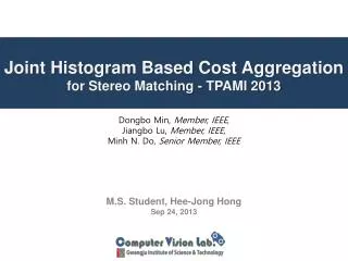
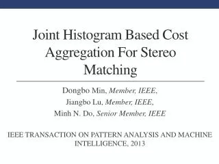
Joint Histogram Based Cost Aggregation For Stereo Matching. Dongbo Min , Member, IEEE , Jiangbo Lu, Member, IEEE , Minh N. Do, Senior Member, IEEE IEEE TRANSACTION ON PATTERN ANALYSIS AND MACHINE INTELLIGENCE, 2013. Outline. Introduction Related Works

E N D
Joint Histogram Based Cost Aggregation For Stereo Matching DongboMin, Member, IEEE, JiangboLu, Member, IEEE, Minh N. Do, Senior Member, IEEE IEEE TRANSACTION ON PATTERN ANALYSIS AND MACHINE INTELLIGENCE,2013
Outline • Introduction • RelatedWorks • Proposed Method:ImproveCostAggregation • ExperimentalResults • Conclusion
Introduction • Goal:Perform efficient cost aggregation. • Solution : Jointhistogram+reduceredundancy • Advantage : Low complexitybutkeephigh-quality.
RelatedWorks N : all pixels (W*H) B : window size L : disparity level • Complexityofaggregation:O(NBL) • Reducecomplexityapproach • Scaleimage[8] • Bilateralfilter[9,10] • Geodesic diffusion[11] • Guidedfilter[12]=>O(NL)
ReferencePaper • [8] D. Min and K. Sohn, “Cost aggregation and occlusion handling with WLS in stereo matching,” IEEE Trans. on Image Processing, 2008. • [9] C. Richardt, D. Orr, I. P. Davies, A. Criminisi, and N. A. Dodgson, “Real-time spatiotemporal stereo matching using the dual-cross- bilateral grid,” in European Conf. on Computer Vision, 2010 • [10] S. Paris and F. Durand, “A fast approximation of the bilateral filter using a signal processing approach,” International Journal of Computer Vision, 2009. • [11] L. De-Maeztu, A. Villanueva, and R. Cabeza, “Near real-time stereo matching using geodesic diffusion,” IEEE Trans. Pattern Anal. Mach. Intell., 2012. • [12] C.Rhemann,A.Hosni,M.Bleyer,C.Rother,andM.Gelautz,“Fast cost-volume filtering for visual correspondence and beyond,” in IEEE Conf. on Computer Vision and Pattern Recognition, 2011
Local Method Algorithm • Cost initialization=>Truncated Absolute Difference => • Cost aggregation=>Weighted filter • Disparity computation=>Winner take all [4,8] [4] K.-J. Yoon and I.-S. Kweon, “Adaptive support-weight approach for correspondence search,” IEEE Trans. Pattern Anal. Mach. Intell., vol. 28, no. 4, pp. 650–656, 2006. [8] D. Min and K. Sohn, “Cost aggregation and occlusion handling with WLS in stereo matching,” IEEE Trans. on Image Processing, vol. 17, no. 8, pp. 1431–1442, 2008.
Improve CostAggregation • New formulation for aggregation • Remove normalization • Joint histogram representaion • Compact representation for search range • Reduce disparity levels • Spatial sampling of matching window • Regularly sampled neighboring pixels • Pixel-independent sampling
New formulation for aggregation • Remove normalization => • Joint histogram representaion
Compact Search Range • Reason • The complexity of non-linear filtering is very high. • Lower cost values do NOT provide really influence. • Solution • Choose the local maximum points. • Only selectDc(<<D) with descending order to be disparity candidates.
Compact Search Range • Cost aggregation => • MC(q):a subset of disparity levels whose size is Dc. N : all pixels (W*H) B : window size D : disparity level O( NBD ) O( NBDc )
Compact Search Range Dc= 5 (Best) Final acc. = 94.2% Dc= 60 Final acc. = 93.7% Dc= 6 Include GT = 91.8% Final acc. = 94.1% • Non-occluded region of ‘Teddy’ image
Spatial Sampling of Matching Window • Reason • A large matching window and a well-defined weighting function leads to high complexity. • Pixels should aggregate in the same object, NOT in the window. • Solution • Color segmentation => time comsuming • Spatial sampling => easy but powerful ● ● ● ● ● ● ●●●●●● ●●● ●●●●●● ●●● ●●●●●● ●●●
Spatial Sampling of Matching Window • Cost aggregation => • S : sampling ratio O( NBDc ) O( NBDc / S2)
Parameter definition N : size of image B : size of matching window N(p)=W×W MD : disparity levels size=D MC : The subset of disparity size=DC<<D S : Sampling ratio Pre-procseeing
ExperimentalResults • Pre-processing • 5*5 Box filter • Post-processing • Cross-checking technique • Weightedmedian filter (WMF) • Device:Intel Xeon 2.8-GHz CPU (using a single core only) and a 6-GB RAM • Parametersetting ( ) = (1.5, 1.7, 31*31, 0.11, 13.5, 2.0)
ExperimentalResults (a) (b) (c) (d)
ExperimentalResults • Using too large box windows (7×7, 9×9) deteriorates the quality, and incurs more computational overhead. • Pre-filteringcan be seen as the first cost aggregation step and serves the removal of noise.
ExperimentalResults The smaller S, the better Fig. 5. Performance evaluation: average percent (%) of bad matching pixels for ‘nonocc’, ‘all’ and ‘disc’ regions according to Dc and S. 2 better than 1
ExperimentalResults The smaller S, the longer The bigger Dc, the longer
ExperimentalResults • APBP : Average Percentage of Bad Pixels
Original images Results Error maps Ground truth
Conclusion • Contribution • Re-formulate the problem withthe relaxed joint histogram. • Reduce the complexity of the joint histogram-based aggregation. • Achieved both accuracy and efficiency. • Futurework • Moreelaborate algorithms for selecting the subset of labelhypotheses. • Estimate the optimal number Dcadaptively. • Extendthemethodtoanopticalflowestimation.