Yee Algorithm (2 Sessions) (1 Task)
Yee Algorithm (2 Sessions) (1 Task). Yee Algorithm. Faraday's law: Ampere's Law: Gauss‘ law for the electric field: Gauss‘ law for the magnetic field:


Yee Algorithm (2 Sessions) (1 Task)
E N D
Presentation Transcript
Yee Algorithm • Faraday's law: • Ampere's Law: • Gauss‘ law for the electric field: • Gauss‘ law for the magnetic field: • In linear, isotropic, non-dispersive materials (i.e., materials having field-independent, direction independent, and frequency-independent electric and magnetic properties): • For materials with isotropic, non dispersive electric and magnetic losses source that attenuate fields via conversion to heat energy: • electric conductivity • equivalent magnetic loss
Yee Algorithm • Maxwell's equations in linear, isotropic, non dispersive, lossy materials: • Out of vector components in Cartesian: • These six coupled PDE forms basis of FDTD numerical algorithm for electromagnetic wave interactions. • FDTD algorithm need not explicitly enforce Gauss‘ law relations indicating zero free electric and magnetic charge. • This can be readily shown that these relations are theoretically a direct consequence of curl equations.
Yee Algorithm • 2-Dimensions Maxwell's Equations: • Assume that structure being modeled extends to infinity in z-direction. • If Eiis also uniform in z-direction, then all derivatives of fields with respect to z must equal zero: • TMz Mode: TEzMode:
Yee Algorithm • Yee Algorithm: • In 1966,Yee originated a set of FDM for time-dependent Maxwell's equations system for lossless materials case. • Fundamentals: • 1. In 3D space every E component is surrounded by four circulating H components, and every H component is surrounded by four circulating E components as: • Attributes Lattice: • finite-difference expressions for space derivatives are central-difference in nature and second-order accurate. • Continuity of Etand Htis naturally maintained across an interface of dissimilar materials if interface is parallel to one of lattice coordinate axes. • For this case, there is no need to specially enforce field boundary conditions at interface. • At beginning of problem, we simply specify material permittivity and permeability at each field component location. • This yields a staircaseapproximation of surface and internal geometry of structure, with a space resolution set by size of lattice unit cell.
Yee Algorithm • Fundamentals (cont.): • 2. Yee algorithm solves for bothE & H fieldsin time and space using coupled equations, rather than solving for field alone with a wave equation. • This is analogous to combined-field integral equation formulation of MM, wherein both E & H boundary conditions are enforced on surface of a material structure. • Using both E & H information, solution is more robust than using either alone (i.e., it is accurate for a wider class of structures). • Both electric and magnetic material properties can be modeled in a straightforward manner. • This is especially important when modeling RCS reduction. • Features unique to each field, such as Htsingularities near edges and corners, azimuthal (looping) H singularities near thin wires, and radial E singularities near points, edges, and thin wires, can be individually modeled if both electric and magnetic fields are available.
Yee Algorithm • Fundamentals (cont.): • 3. Fieldscomponents in time, in what is termed a leapfrog arrangement as illustrated in: • All of E computations in modeled space are completed and stored in memory for a particular time point using previously stored Hdata. • All of H computations in space are completed and stored in memory using E data just computed. • The cycle begins again with re-computation of E components based on newly obtained H. • This process continues until time-stepping is concluded. • Leapfrog time-stepping is fully explicit, thereby avoiding problems involved with simultaneous equations and matrix inversion. • finite-difference expressions for time derivatives are central-differencein nature and second-order accurate. • time-stepping algorithm is non-dissipative. • That is, numerical wave modes propagating in the mesh do not spuriously decay due to a nonphysical artifact of time-stepping algorithm.
Yee Algorithm • Finite Differences and Notation: • For example: • FDTD Model: • Since Exvalues at time-step nare not assumed to be stored in computer's memory (only previous values of Exat time step n -1/2 are assumed to be in memory). • A very good way to estimate such termsis a semi-implicit approximation:
Yee Algorithm • By combination recent formulas and multiplying both sides by Δt: • By rearranging: • Dividing both sides by:
Yee Algorithm X + • Similarly, FDTD approximation for Eycomponent can be derived as: • Similarly, FDTD approximation for Ezcomponent can be derived as: X +
Yee Algorithm • Similarly, FDTD approximation for Hx, Hy &Hzcomponent can be derived as:
Yee Algorithm • Continuous Variation of Material Properties: • For such media, it is desirable to define and store following constant, to update coefficients for each field vector component before time stepping begins. • For E fields: For H fields: • For a cubic lattice: • Therefore: 1. 2. 3. 1. 2. 3.
Yee Algorithm • FDTDexpressions of fields can now be rewritten more simply as:
Yee Algorithm • Space Region with a Finite Number of Distinct Media: • This can be done by defining an integer array, MEDIA(i, j, k), for each set of field vector components. • This array stores an integer "pointer" at each location of such a field component in space lattice, enabling the proper algorithm coefficients to be extracted. • FDTD expressions of fields can now be rewritten more simply as: • By a similar manner: … … … … …
Yee Algorithm • Alternative Finite-difference Grids: • Cartesian Grids: • Two Cartesian grids that are alternatives to Yee's arrangement: • First depicts un-staggered in which field componentsare collocated at a single set of grid-cell vertices. • Second depicts staggered in which all E components are collocated at a distinct set of grid-cell vertices. • Applying second-order-accurate central space differences to TMzmode equations for first case havingσ=0:
Yee Algorithm • Alternative Finite-difference Grids (cont.): • Applying second-order-accurate central space differences to TMzmode equations for second case havingσ=0:
Yee Algorithm • Alternative Finite-difference Grids (cont.): • Hexagonal Grids: • Proposed regular hexagonal grids reduce numerical phase velocity anisotropy well below that of Yee's Cartesian mesh [4]. • For un-staggered, collocated hexagonal grid with a loss less material:
Yee Algorithm • Hexagonal Grids (cont.): • For staggered hexagonal grid with a loss less material: • Number of field unknowns for staggered is 33% more than that for un staggered. • But discretization is simpler and number of total operations is less by approximately 50%. • Numerical dispersion of two hexagonal cases shows that velocity-anisotropy errors are 1/200th and 1/1200th, respectively, that of second-order accurate Yee grid for a sampling density of 1/20λ. • This represents a large potential advantage in computational accuracy for hexagonal grids.
Practical Applications • Wave scattering using FDTD: • Wave scattering using FDTD method will cover: • Yee’s Algorithm, • Accuracy & Stability, • Absorbing Boundary Conditions (ABC), • Initial Fields, • Programming Aspects, • Yee’s Algorithm: • In an isotropic medium: • Using: • Where: =
Practical Applications • Wave scattering using FDTD (cont.): • Using central difference approximation: • Using Yee’s lattice, explicit finite difference approximation: Positions of field components in a unit cell of the Yee’s lattice
Practical Applications • Wave scattering using FDTD (cont.):
Practical Applications • Wave scattering using FDTD (cont.): • For 3D case, scattered waves have all six field components. • With assuming δt=δ/2c, If lattice occupies: • Truncation conditions (Boundary conditions) are: • For plane i=1/2: • For plane i=Imax+1/2: • For plane j=0: • For plane j=Jmax: • For plane k=0: • For plane k=Kmax: … … … …
Practical Applications • Wave scattering using FDTD (cont.): • Accuracy and Stability: • To accuracy, spatial increment δ must be small compared to the wavelength (usually ≤ λ/10). • Or small than minimum dimension of the scatterer. • To stability, the time increment Δt must satisfy following stability condition: • Where umax is maximum wave velocity within model. • Since we are using a cubic cell having x=y=z=δ: • Where n is number of space dimensions. • For practical reasons, it is best to choose ratio of time increment to spatial increment as large as possible.
Practical Applications • Wave scattering using FDTD (cont.): • Lattice Truncation Conditions: • A basic difficulty in FDTD, to scattering problems, is that domain is open or unbounded. • Since no computer can store an unlimited amount of data, applying FDTD is impractical. • We must limit the extent of our solution region. • In other words, an artificial boundary must been forced, as shown in: • Solution region must be large enough to enclose scatterer, and suitable boundary conditions on artificial boundary must be used to simulate extension of solution region to infinity. … y=δ y=2δ y=3δ y=(J-1)δ • Outer boundary conditions of this type have been called radiation conditions, or absorbing boundary conditionsor lattice truncation conditions. • Several types of boundary conditions have been proposed such as Taflove’sboundarycondition. • Taflove’sboundarycondition allow excellent overall accuracy and numerical stability even when lattice truncation planes are positioned no more than 5δ from surface of scatterer. • Conditions relate in a simple way values of the field components at truncation planes to field components at points one or more δ within lattice.
Practical Applications • Lattice Truncation Conditions (cont.): • For example for 1D wave propagation have Ezand Hx components in ±y directions. • Assuming a time step of δt=δy/c, which is maximum allowed by stability condition. • If lattice extends from y=0 to JΔy, with Ez component at end points, truncation conditions are: • With these lattice conditions, all possible ±y-directed waves are absorbedat y=0 & J without reflection. • That is assumes free-space propagation. • To simulate lattice truncation in a dielectric medium of refractive index m: … y=1 y=0 y=2δ y=3δ y=(J-1)δ y=δ • This is the base of travelling wave concept having VSWR=0
Practical Applications • Wave scattering using FDTD (cont.): • Initial Fields: • Initial field components are obtained by simulating: • Either an incident plane wave pulse. • Or single-frequency plane wave. • For 3D case, a typical wave source condition at plane y=js (near y=0) is: • Value of sinusoid wave (with f=f0) is added to value of Enzby FDTD formula. • Plane wave source turned on at t=0. • Propagation of waves from this source is simulated by Δt, by implementing Yee’s FDTD algorithm. • Incident wave is tracked as it first propagates to scatterer and then interacts with it via surface-current excitation, diffusion, penetration, and diffraction. • Δt is continued until sinusoidal steady state is achieved at each point. • From experience, number of Δt needed to reach steady state can be greatly reduced by introducing a small isotropic conductivity σext within region. • This causes fields to converge more rapidly to expected steady state condition. updated field source Computed by FDTD
Practical Applications • Programming Aspects: • Since most EM scattering problems involve μr=1, quantity δt / μ(i,j,k) δ can be assumed constant for all (i, j, k). • Therefore Nine multiplications per unit cell per time required by Yee’s algorithm can be reduced to six multiplications, thereby reducing computer time. • Following constants introduced by Taflove [31, 35, 44]: • Where m=MEDIA(i,j,k)is an integer referring to dielectric or conducting medium type at location (i,j,k). • For example, for a solution region comprising of three different homogeneous media shown in Figure, m=1, 2, 3. • mshould not be confused with refractive index of medium • In addition to the above constants, Taflove defined proportional electric field as: introduced in previous slides typical inhomogeneous solution region
Practical Applications • Programming Aspects (cont.): • Thus modified Yee’s algorithm, for easy programming, is simplified as:
Practical Applications • Programming Aspects (cont.): • Relationship between original and modified algorithms is shown in table: • This modification eliminates need for computer storage of separate µ and σarrays. • Therefore only a MEDIA array which specifies type-integer of dielectric or conducting medium at location of each electric field component in lattice need be stored. • Also the programming problem of handling half integral values of i,j,khas been eliminated. • With modified algorithm, we determine scattered fields. • Let solution region, completely enclosing scatterer, be defined by 0<i<Imax, 0<j<Jmax, 0<k<Kmax. • At t≤0, program is started by setting all field components at grip points equal to zero:
Practical Applications at all grid points in solution region • Programming Aspects (cont.): • For 0<i<Imax, 0<j<Jmax, 0<k<Kmax, if we know: • We can determine new Hx(i,j,k) everywhere as: • Other field components can be find by using modified Yee’s formula and lattice truncation conditions. • Plane wave source is activated at first time step t=Δt, and left on during entire run. • Time stepping is continued for t=NmaxΔt, where Nmaxis chosen large enough that sinusoidal steady state is achieved. • In obtaining steady state solutions, program must not be left for too long (i.e., Nmaxshould not be too large), otherwise imperfection of boundary conditions causes model to become unstable. modified node numbering
Practical Applications • Example: • Consider scattering of +y-directed plane wave of frequency 2.5GHzby a uniform, circular, dielectric cylinder of radius 6cm. • We assume that cylinder is infinite in z-direction and that incident fields do not vary along z. • Thus ∂/∂z=0 and problem is reduced to two-dimensional scattering of incident wave with only Ez, Hx, and Hycomponents. • Our objective is to compute oneof components, such as Ez, at points within cylinder. • Assuming a lossless dielectric with: • Solution: • Hence: • Assumptions:
Practical Applications • Solution (cont.): • Maxwell’s Equations: • Axis as passing through point (i,j)=(25.5, 24.5) allows symmetry condition to be imposed at line i=26, i.e.,: • Soft grid truncation conditions are applied at j=0, 49 and i=1/2, i.e.,: • Grid points (i,j) internal to cylinder, determined by: FDTD model of cylindrical dielectric scatterer
Practical Applications • A FORTRAN program has been developed by Bemmel based on ideas expounded above. • A similar but more general code is THREDE developed by Holland. • Program starts by setting all field components at grid points equal to zero. • A plane wave source as: • is used to generate incident wave at j=2 and n=1, first time step, and left on during entire run. • Program is time stepped to t=Nmaxδt, where Nmaxis large enough that sinusoidal steady state is achieved. • Since f=2.5GHz, wave period T=1/f=400ps=80δt. • Hence Nmax=500=6.25T/δt is sufficient to reach steady state. thus process is terminated after 500δt • Results, including exact solution using series expansion, for 460≤n≤500 are shown in: j j • LN6T1: Implement FDTD code to • 1. Generate a 1D plane wave source and apply Yee algorithm without dielectric cylinder and animate solution. • 2. Generate a 2D plane wave source and apply Yee algorithm without dielectric cylinder and animate solution. • 3. Generate results of the example and compare with exact solution.
Practical Applications • Example: • Consider penetration of +y-directed plane wave of frequency 2.5GHzby a uniform, dielectric sphere of radius 4.5cm. • Assume that incident wave has only Ez and Hx components. • Repeat previous example . • Solution: • Problem is similar to previous example except that it is 3D and more general. • FDTD model of dielectric sphere is shown: • This choice of grid size implies that radius of sphere is 4.5/0.3=15 units. • Grid points (i,j,k) internal to sphere are determined by: • Rather than assigning σ=0to points external to sphere, a value σ=0.1mho/m is assumed to reduce spurious wave reflections. • FORTRAN code is shown in the book. • With dimensions and constitutive parameters of sphere specified as input data, program is developed based on following steps:
Practical Applications • Example (cont.): • Step 1. Compute parameters of each medium using: m=1,2 and : • Step 2. Initialize field components. • Step 3. Use FDTD equations to generate field components. • This is the heart of the program. taking following steps: • 1. Calculate actual values of grid point (x,y,z) using relationship in presentedTable. • This will be needed later to identify ε & µat that point using subroutine MEDIA. • 2. Apply soft lattice truncation conditions in previous presented equation at appropriate boundaries. • Notice that some of truncation conditions are not necessary in this case because we restrict solution to 1/4 of sphere due to geometrical symmetry. • For example, at k=19: • 3. Apply FDTD algorithm introduced previous slides. • 4.Activate plane wave source, i.e., where js=3 or any plane near y=0. • 5. Time step until steady state is reached. • Step 4. Obtain maximum absolute values (envelopes) of field components in last λ/2 and output results.
Practical Applications • Example (cont.): • Results of the program illustrated in: • Values of |Ey| and |Ez| near sphere axis are plotted against jfor observation period 460 ≤n ≤500. • Computed results are compared with Mie’s exact solution. • Programming codes for calculating exact solution is also found in Bemmel’s work [80]. • LN6T2: (Optional) • Implement FDTD code to • 1. Generate a 2D plane wave source only and animate the solution. • 2. Generate results of the example and compare with exact solution. • Generate results to plot RCS a PEC sphere in regions of Rayleigh, Mie & Optic as shown in the literatures. • Generate results to plot RCS a dielectric sphere in three region as shown in literatures.