Download
1 / 25
250 likes | 355 Views
Computational BioMedical Informatics. SCE 5095: Special Topics Course Instructor: Jinbo Bi Computer Science and Engineering Dept. Course Information. Instructor: Dr. Jinbo Bi Office: ITEB 233 Phone: 860-486-1458 Email: jinbo@engr.uconn.edu

E N D
Computational BioMedical Informatics SCE 5095: Special Topics Course Instructor: Jinbo Bi Computer Science and Engineering Dept.
Course Information • Instructor: Dr. Jinbo Bi • Office: ITEB 233 • Phone: 860-486-1458 • Email:jinbo@engr.uconn.edu • Web: http://www.engr.uconn.edu/~jinbo/ • Time: Tue / Thu. 3:30-4:45pm • Location: CAST 201 • Office hours: Tue. 2:30-3:30pm • HuskyCT • http://learn.uconn.edu • Login with your NetID and password • Illustration
Summary of topics in clustering • Discussed different types of clusterings, and different cluster types • Introduced k-means • Introduced hierarchical clustering, particularly the bottom-up approaches, focused on intra-cluster distance/similarity design • Introduced spectral clustering, local behaviors • Started to look at a medical problem where clustering techniques can be applied
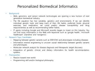
Application in medical informatics • Anatomy of the heart • Cardiac ultrasound videos (clips) • 2-D view recognition problem • Diagram of building an informatics system • Preprocessing (normalization, fan detection) • Feature calculation • Clustering • Validation
Planes of the Heart Short-axis view Long-axis view Apical 4-chamber
Ultrasound Clips • Parasternal long-axis view, parasternal short-axis view, apical 4-chamber view, apical 2-chamber view • A healthy heart http://www.youtube.com/watch?v=7TWu0_Gklzo&feature=related • An abnormal heart (dilated cardiomyopathy) http://www.youtube.com/watch?v=37KDMNiV3AU&feature=related • Abnormal heart (hypertrophic cardiomyopathy) http://www.youtube.com/watch?v=QSQx8c8UkUk&feature=fvw • Abnormal heart (Ruptured papillary muscle) http://www.youtube.com/watch?v=gUdegG0-Shc&feature=related
Data Preprocessing • Fan Detection • Even images from a single vendor have different fan areas • ATL has four different fan sizes • Acuson has different image resolutions • etc. • Intensity Normalization • We convert all images to grayscale • Basic linear normalization: • I’ = I / (U – L) • Smoothing • Performed during feature extraction
Fan Detection: Different Fan Areas Large Regular Small Tiny
Fan Detection Step One Step Two Largest connected region approach Step Three Step Four Step Five Step Six
Fan Detection Largest connected region approach
Fan Detection Largest connected region approach
Feature Extraction • Basic Gradients • Other Gradient Features • Peaks • Pixel Intensity Histograms • Not very useful • Statistical Features • Mean, standard deviation, and statistical moments of pixel intensities in the average frame • Raw Pixel Intensities • Alpha Features
Basic Gradients • Find sum of the magnitudes of the gradients in the x, y, and z directions • These features characterize • Horizontal and vertical structure (x and y gradients) • Motion (z gradient) xgrad = ygrad = 0; for each frame { find gradient in x-direction; xsum = sum of magnitudes of all gradients in mask area; xgrad = xgrad + xsum; find gradient in y-direction; ysum = sum of magnitudes of all gradients in mask area; ygrad = ygrad + ysum; }
Other Gradient Features • XZ and YZ Gradients • Real Gradients (x, y, and z) • Gradient Sums (x+y, x+z, y+z) • Gradient Ratios (x:y, x:z, y:z) • Gradient Standard Deviations (x, y, and z)
Peak Features • Features that characterize the number of horizontal and vertical walls in an image • Potentially useful for distinguishing between apical two-chamber and apical four-chamber views. • Very sensitive to noise Take average of all frames to produce a single image matrix Sum up over all rows of matrix Normalize by the number of fan pixels in each column Smooth this vector to remove peaks due to noise xpeaks = the number of maxima in the vector
a4c a2c min 1 3 max 9 6 mean 3.72 4.48 median 3 4 Peak Results
Data for Clustering f1 f2 f3 • 0.1 1.2 3.4 • 0.9 3.5 5 ….. ….. ……
Next class • Lab Assignment (no lecture) • Classroom changes to • ITEB 138 • Instructor and TA available for any questions about Matlab