6.1 day 2
6.1 day 2. Euler’s Method. Leonhard Euler made a huge number of contributions to mathematics, almost half after he was totally blind. . (When this portrait was made he had already lost most of the sight in his right eye.). Leonhard Euler 1707 - 1783.


6.1 day 2
E N D
Presentation Transcript
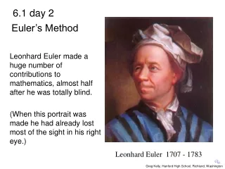
6.1 day 2 Euler’s Method Leonhard Euler made a huge number of contributions to mathematics, almost half after he was totally blind. (When this portrait was made he had already lost most of the sight in his right eye.) Leonhard Euler 1707 - 1783 Greg Kelly, Hanford High School, Richland, Washington
(function notation) (base of natural log) (pi) (summation) (finite change) It was Euler who originated the following notations: Leonhard Euler 1707 - 1783
We will practice with an easy one that can be solved. Initial value: There are many differential equations that can not be solved. We can still find an approximate solution.
This is called Euler’s Method. It is more accurate if a smaller value is used for dx. It gets less accurate as you move away from the initial value.
Y= The TI-89 has Euler’s Method built in. Example: We will do the slopefield first: MODE Graph….. 6: DIFF EQUATIONS We use: y1 for y t for x
WINDOW t0=0 tmax=150 tstep=.2 tplot=0 xmin=0 xmax=300 xscl=10 ymin=0 ymax=150 yscl=10 ncurves=0 diftol=.001 fldres=14 Y= GRAPH MODE Graph….. 6: DIFF EQUATIONS We use: y1 for y t for x not critical
WINDOW t0=0 tmax=150 tstep=.2 tplot=0 xmin=0 xmax=300 xscl=10 ymin=0 ymax=150 yscl=10 ncurves=0 diftol=.001 fldres=14 GRAPH
I and change Solution Method to EULER. Press WINDOW If tstep is larger the graph is faster. If tstep is smaller the graph is more accurate. Y= GRAPH While the calculator is still displaying the graph: yi1=10 tstep = .2
F8 F3 You can also investigate the curve by using . Trace To plot another curve with a different initial value: Either move the curser or enter the initial conditions when prompted.
WINDOW t0=0 tmax=10 tstep=.5 tplot=0 xmin=0 xmax=10 xscl=1 ymin=0 ymax=5 yscl=1 ncurves=0 Estep=1 fldres=14 Y= GRAPH Now let’s use the calculator to reproduce our first graph: We use: y1 for y t for x I Change Fields to FLDOFF.
F3 Use to confirm that the points are the same as the ones we found by hand. Trace TblSet Press and set: Press Table
Press Table This gives us a table of the points that we found in our first example.
The calculator also contains a similar but more complicated (and more accurate) formula called the Runge-Kutta method. You don’t need to know anything about it other than the fact that it is used more often in real life. This is the RK solution method on your calculator. The book refers to an “Improved Euler’s Method”. We will not be using it, and you do not need to know it. p