Download
1 / 38
380 likes | 465 Views
Explore solar phenomena using EIS advanced spectroscopy tools for in-depth analysis of active regions, flares, CMEs, and more in this preliminary science plan.

E N D
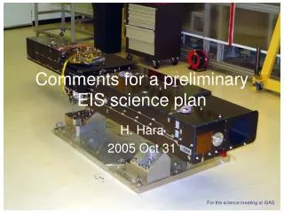
Comments for a preliminary EIS science plan H. Hara 2005 Oct 31 For the science meeting at ISAS
Observables w • Line intensity • Line shift by Doppler motion • Line width temperature, nonthermal motion Information from selected two line ratio • Temperature • Density
EIS Slit/Slot • Four slit selections available • EUV line spectroscopy - 1 arcsec 512 arcsec slit for the best image quality - 2 arcsec 512 arcsec slit for a higher throughput • EUV Imaging (overlappogram; velocity info. overlapped) - 40 arcsec 512 arcsec slot for imaging with little overlap -250 arcsec 512 arcsec slot for hunting transient events
512 pixels EIS Spectral Windows Spectral window W H
EIS Data Processing Line intensity ratio N density
CDS vs EIS EIS has • A larger effective area: AEIS ~ 10 ACDS • Higher spatial resolution: EIS: 2 arcsec CDS: > 5arcsec (out-of-focus) • Higher spectral resolution: REIS 3 RCDS measurement of emission-line width • Larger FOV (EWNS): EIS 590”x512” CDS 240”240” • Higher telemetry rate • High compression performance: EIS DPCM/JPEG CDS loss-less • Flare-temperature lines • Automatic observation controls: Automatic exposure control, XRT flare response, EIS flare trigger EIS event trigger, anti-solar rotation compensation
EIS science plan • EIS core science program http://www.mssl.ucl.ac.uk/www_solar/solarB/core.htm Category: Active Regions, Quiet Sun, Flares, CME, LSS • EIS initial science plan (for the first 3 months) http://www.mssl.ucl.ac.uk/www_solar/solarB/eis_swg1.htm Core lines: Ca XVII 193, Fe XII195, He II 256 Topics: AR heating, QS and CH, Flare Hara is thinking that the plan has not yet been optimized.
AR • (i) connect the photospheric velocity field to signatures of coronal heating observed in the corona. This will be carried out on other coronal brightenings, such as bright points. • (ii) search for evidence of waves and loop oscillations in loops. Use EIS observations for coronal seismology. • (iii) study dynamic phenomena within active region loops. Discriminate between siphon flows, bi-directional flows and turbulence.
QS • (i) link quiet Sun brightenings and explosive events to the magnetic field changes in the network and inter-network to understand the origin of these events. We will search for responses to small changes in the photospheric magnetic and velocity fields. • (ii) determine the variation of explosive events and blinkers with temperature. • (iii) search for evidence of reconnection and flows at junctions between open and closed magnetic field at coronal hole boundaries. • (iv) determine the impact of quiet Sun events on larger scale structures within the corona. • (v) determine physical size scales with generally diffuse quiet Sun coronal plasmas using density diagnostics.
Flare • (i) determine the source and location of flaring and identify the source of energy for flares. EIS will measure the velocity fields and observe coronal structures with temperature information. This information will help us address the flare trigger mechanism. • (ii) detection of reconnection inflows, outflows and the associated turbulence which play the pivotal role in flare particle acceleration.
CME • (i) determine the location of dimming (and the subsequent velocities) in various magnetic configurations. We will determine the magnetic environment that leads to a coronal mass ejection and measure the low altitude component of the coronal mass ejection mass budget. • (ii) The situations to be studied include filaments, flaring active regions and trans-equatorial loops.
LLS • (i) determine the temperature and velocity structure in a coronal streamer • (ii) determine the velocity field andtemperaturechange of a trans-equatorial loop, and search for evidence of large-scale reconnection. • (iii) using a low latitude coronal hole, search for the source of the fast solar wind.
EIS Initial Science Plan • Core line list: we will include 3 lines in ALL studies He II 256, Fe XII 195, Ca XVII 192.8 • Flare trigger/dynamics:spatial determination ofevaporationand turbulence in flares • AR heating:spatial determination of the velocity field in active region loops over a range of temperatures • QS & CH:determination of the relationship between the various categories of quiet Sun brightenings (e.g explosive events and blinkers) both in the quiet Sun and coronal holes. EIS has the spatial and velocity resolution to solve this mystery. • The observing time will be split evenly between the topics. If there is an active region we will track it otherwise we will observe quiet Sun and coronal holes for long periods of time (at least 12 hrs). • When there is an active region we will track it, and if there is highly sheared magnetic field then we will go into flare trigger mode to respond to XRT's trigger. • If there are no active regions but there is a quiet prominence we concentrate on this.
EIS Data Flow Data compression DPCM(loss less) or 12bit-JPEG Small spectral window (25 max) CCD Readout Electronics 2Mbps max 1.3 Mbps EIS ICU S/C MDP control 260 kbps max for short duration, 45 kbps average Large hardware CCD window Observation table 1 slit obs. 40 slot obs. 250 slot obs. Spec.width 16 40 250 Spatial width 256 512 256 No. of lines 8 4 4 Compression* 25% 20 % 20% Cadence 3 sec 6 sec 20 sec Rate 42.7 kbps 42.7 kbps 40 kbps Average rate depends on number of downlink station. Telemetry data format *for 16 bit/pixel data 13 min cadence for 44 rastering
EIS Data Rate Data rate = CCSDS format data size / cadence ~ [EIS data size to MDP] * [Compression Ratio] / Cadence EIS data size to MDP = total sum of software windows = (window width)i * (window height)i Compression ratio = compressed data size/ input data size to MDP Cadence = setup time + exposure duration [+ data transfer time] High data rate Low data rate SW width/SW height/Number of SW small large JPEG compression Large Q-factor Small Q-factor (Large compression error) (Small compression error) Exposure duration Long Short
Density Sensitive Line Ratio Density sensitive line ratio with two forbidden lines Filling factor of coronal loop will be estimated in 2 arcsec resolution. CHIANTI is used for this estimate. Fe XI line ratios 182.17/188.21 and 184.80/188.21 will also be useful. (Keenan et al. 2005)
AR Heating • Line list 1: Fe XII195 • Line list 2: Fe XI188, Fe XXIV192, Fe XII195, Fe XIII202, Fe XIII203, HeII256,Fe XV284 • Line list 3: LL2+ FeX184,FeVIII185,FeXII186,CaXVII193,FeXVI263,FeXIV264,FeXIV274, • SiVII275
Flare • Line list 1: Core (Fe XII195, CaXVII193, HeII256), FeX184,Fe XXIV192,FeXV284 • Line list 2: Core, FeX, FeXV284, FeXXIV+FeXXIII+FeXXII (253) for 266” slit, 5 segments
Quiet Sun • Line list 1: Core (Fe XII195, CaXVII193, HeII256), FeX184,FeVIII185, Fe XII186 FeXI188,FeXXIV192,FeXII196,FeXIII202, Fe XIII203, FeXVI263,S X264 FeXIV264,SiVII275,FeXV284 • Line list 2: Fe XII195,HeII256,FeXV284 • Line list 3: whole CCD area
EIS Sensitivity Detected photons per 11 area of the sun per 1 sec exposure. AR: active region
EIS CAL data • EIS end-to-end calibration was performed at RAL. One of CAL images (md_data.028; given by J. Mariska ) was used to check the MDP compression capability. • The following four images are taken from md_data.028. • CAL1: x= 860: 860+127, y=90:90+255 ; on CCD11 • CAL2: x=1270:1270+127, y=90:90+255; on CCD10 • CAL3: x=2940:2940+127, y=90:90+255; on CCD01 • CAL4: x=3670:3670+127, y=90:90+255; on CCD00 • CAL 2,3,and 4 were set in the EIS simulator PC during FM MDP integration for testing of compression. CAL4 CAL3 CAL2 CAL1
MDP compression parameters • Bit compression table7 parameters. • A= 1877.50, B = 341.00, C= -6692998, Nc=2048. • 12bit_data = 14bit_data for value Nc 12bit_data = round( A + sqrt(B*14bit_data +C) ) for value>Nc • No bit & image compression : 0x0000 • No bit & DPCM : 0x0328; extraction of lower 12bits data • Bit table7 & DPCM : 0x3B28 • Bit table 7 & JPEG (Q=98) : 0x3F28 • Bit table 7 & JPEG (Q=90) : 0x3F29 • Bit table 7 & JPEG (Q=75) : 0x3F2A • Bit table 7 & JPEG (Q=50) : 0x3F2B • Bit table 7 & JPEG (Q=95) : 0x3F2C • Bit table 7 & JPEG (Q=92) : 0x3F2D • Bit table 7 & JPEG (Q=85) : 0x3F2E JPEG Q-tables are shared with • Bit table 7 & JPEG (Q=65) : 0x3F2F SOT and XRT teams.
Q=98 CAL2 JPEG data size Spec: 65536 bytes 15058 bytes Comp. Factor = 4.35 or 23.0 % of original data Original Line:150 256 pixels 128 pixels 128x256x2 = 65536 bytes
Q=95 CAL2 JPEG data size Spec: 65536 bytes 10096 bytes Comp. Factor = 6.49 or 15.4% of original data Original Line:150 256 pixels 128 pixels 128x256x2 = 65536 bytes
Q=92 CAL2 JPEG data size Spec: 65536 bytes 7252 bytes Comp. Factor = 9.04 or 11.1% of original data Original Line:150 256 pixels 128 pixels 128x256x2 = 65536 bytes
Q=90 CAL2 JPEG data size Spec: 65536 bytes 6368 bytes Comp. Factor = 10.3 or 9.7% of original data Original Line:150 256 pixels 128 pixels 128x256x2 = 65536 bytes
Q=85 CAL2 JPEG data size Spec: 65536 bytes 4832 bytes Comp. Factor = 13.6 or 7.4% of original data Original Line:150 256 pixels 128 pixels 128x256x2 = 65536 bytes
Q=75 CAL2 JPEG data size Spec: 65536 bytes 3588 bytes Comp. Factor = 18.3 or 5.5% of original data Original Line:150 256 pixels 128 pixels 128x256x2 = 65536 bytes
Q=65 CAL2 JPEG data size Spec: 65536 bytes 2962 bytes Comp. Factor = 22.1 or 4.5% of original data Original Line:150 256 pixels 128 pixels 128x256x2 = 65536 bytes
Q=50 CAL2 JPEG data size Spec: 65536 bytes 2496 bytes Comp. Factor = 26.3 or 3.8% of original data Original Line:150 256 pixels 128 pixels 128x256x2 = 65536 bytes
JPEG: Compression Error X: signal – offset [DN] ; offset~ 500 Y: decomp( comp( Original ) ) – Original [DN] DN17nm DN29nm
Line Parameters by Gaussian Fitting Data: CAL2 Line 1 Line 2 Data Comp. Peak Center FWHM Peak Center FWHM size factor (DN) (pixel) (pixel) (DN) (pixel) (pixel) (bytes) Raw 176.0 75.75 2.32 87.6 87.15 2.20 65536 1.00 =20 =0.10 =0.25 =15 =0.15 =0.33 ( 3.7km/s) ( 9.2km/s)( 5.6km/s) ( 12km/s) DPCM 176.0 75.75 2.32 87.6 87.15 2.20 20436 3.21 JPEG Q=98 176.8 75.74 2.30 86.3 87.15 2.21 15058 4.35 Q=95 176.5 75.74 2.32 84.7 87.15 2.22 10096 6.49 Q=92 178.5 75.76 2.29 89.9 87.20 2.10 7252 9.04 Q=90 180.3 75.76 2.11 91.9 87.19 2.11 6368 10.29 Q=85 175.5 75.78 2.30 87.0 87.12 2.38 4832 13.56 Q=75 174.9 75.75 2.24 85.6 87.24 2.22 3588 18.27 Q=65 180.7 75.75 2.23 85.3 87.19 2.30 2962 22.13 Q=50 178.7 75.76 2.24 82.5 87.19 2.19 2496 26.26
Line Parameters by Gaussian Fitting Data: CAL3 Line 1 Line 2 Data Comp. Peak Center FWHM Peak Center FWHM size factor (DN) (pixel) (pixel) (DN) (pixel) (pixel) (bytes) Raw 2383.37 62.08 2.56 513.1 91.77 2.67 65536 1.00 =68 =0.03 =0.08 =31 =0.07 =0.17 ( 1.1km/s) ( 2.9km/s)( 2.6km/s) ( 6.3km/s) DPCM 2383.7 62.08 2.56 513.1 91.77 2.67 21406 3.06 JPEG Q=98 2385.8 62.08 2.56 512.7 91.77 2.66 16828 3.89 Q=95 2382.4 62.08 2.57 514.3 91.77 2.64 11784 5.56 Q=92 2381.7 62.08 2.57 518.5 91.78 2.60 8764 7.48 Q=90 2371.1 62.08 2.59 512.4 91.77 2.65 7818 8.38 Q=85 2378.4 62.09 2.58 522.2 91.79 2.66 6042 10.85 Q=75 2354.3 62.09 2.60 516.3 91.80 2.61 4432 14.79 Q=65 2329.5 62.09 2.62 522.1 91.78 2.62 3714 17.65 Q=50 2334.1 62.09 2.62 522.0 91.78 2.59 3110 21.07
CDS vs EIS EIS has • A larger effective area: AEIS ~ 10 ACDS • Higher spatial resolution: EIS: 2 arcsec CDS: > 5arcsec (out-of-focus) • Higher spectral resolution: REIS 3 RCDS measurement of emission-line width • Larger FOV (EWNS): EIS 590”x512” CDS 240”240” • Higher telemetry rate • High compression performance: EIS DPCM/JPEG CDS loss-less • Flare-temperature lines • Automatic observation controls: Automatic exposure control, XRT flare response, EIS flare trigger EIS event trigger, anti-solar rotation compensation
Summary • Use of JPEG compression is unavoidable even for EIS spectroscopic observations. • Need more investigation on JPEG performance for a high data rate.