Download

1 / 63
630 likes | 891 Views
Measurement and Interpretation of Elasticities. Chapter 5. Discussion Topics. Own price elasticity of demand Income elasticity of demand Cross price elasticity of demand Other general properties How can we use these demand elasticities. 2. Key Concepts Covered….

E N D
Discussion Topics • Own price elasticity of demand • Income elasticity of demand • Cross price elasticity of demand • Other general properties • How can we use these demand elasticities 2
Key Concepts Covered… • Own price elasticity = %Qi for a given%Pi, ηii • i.e., the effect of a change in the price for hamburger on hamburger demand: ηHH = %QH for a given%PH • Cross priceelasticity = %Qifor a given %Pj, ηij • i.e., the effect of a change in the price of chicken on hamburger demand: ηHC = %QH for a given%PC • Incomeelasticity = %Qifor a given%Income, ηiY • i.e., the effect of a change in income on hamburger demand: ηHY = %QH for a given%PY Pages 70-76 3
Key Concepts Covered… • Arc elasticity = elasticity estimated over a range of prices and quantities along a demand curve • Point elasticity = elasticity estimated at a point on the demand curve • Price flexibility = reciprocal (the inverse) of the own price elasticity • %Pifor a given%Qi Pages 70-76 4
Own Price Elasticity of Demand Own price elasticity of demand Percentage change in quantity demanded (Q) ηii= Percentage change in own price (P) $ Point Elasticity Approach: Single point on curve Own price elasticity of demand Pa Pb Q Qb Qa Q = (Qa – Qb) P = (Pa – Pb) • The subscript • a stands for after price change • bstands for before price change 6 Pages 70-72
Own Price Elasticity of Demand Own price elasticity of demand Specific range on curve Percentage change in quantity ηii= $ Percentage change in own price Pa Arc Elasticity Approach: Pb Own price elasticity of demand Q Qa Qb where: P= (Pa + Pb) 2 Q= (Qa + Qb) 2 Q = (Qa – Qb) P = (Pa – Pb) Equation 5.3 Avg Price • The subscript • a stands for after price change • bstands for before price change Avg Quantity Page 72 7
Interpreting the Own Price Elasticity of Demand Note: The %Δ in Q is in terms of the absolute value of the change 8 Page 72
Demand Curves Come in a Variety of Shapes $ Perfectly Inelastic ∆P Perfectly Inelastic: A price change does not change quantity purchased Perfectly Elastic Q 10 Page 72
Demand Curves Come in a Variety of Shapes $ Inelastic Demand ∆P ∆P Elastic Demand Q ∆Q ∆Q 11 Page 73
Demand Curves Come in a Variety of Shapes $ Elastic where –%Q > % P Unitary Elastic where –%Q = % P Inelastic where –%Q < % P Q 12 Page 73
Example of Arc Own-Price Elasticity of Demand • Unitary elasticity • –% Change in Q = % Change in P • ηii= –1.0 Page 73 13
Elastic demand Inelastic demand Page 73 14
Elastic Demand Curve $ • With the price decrease from Pb to Pa • What happens to producer revenue? Pb Pa Q 0 Qb Qa 15
Elastic Demand Curve $ Results in a larger % increase in quantity demanded Pb Cut in price Pa Q 0 Qb Qa 16
Elastic Demand Curve • Producer revenue (TR) = price x quantity • Revenue before the change (TRb) is Pb x Qb • Represented by the area 0PbAQb • Revenue after the change is (TRa) is Pa x Qa • Represented by the area 0PaBQa $ C A Pb B Pa Q 0 Qa Qb 17
Elastic Demand Curve • Change in revenue (∆TR) is TRa – TRb • → ∆TR = 0PaBQa– 0PbAQb • → ∆TR = QbDBQa – PaPbAD • →TR ↑ • %Q ↑ is greater than %P ↓ $ Red Box Purple Box C A Pb D B Pa • When you have elastic demand • ↑ in price → ↓ total revenue • ↓ in price → ↑ total revenue Q 0 Qa Qb 18
Inelastic Demand Curve $ Pb Cut in price Pa Results in smaller % increase in quantity demanded Q Qb Qa 19
Inelastic Demand Curve $ • With price decrease from Pb to Pa • What happens to producer revenue? Pb Pa Q Qb Qa 20
Inelastic Demand Curve • Producer revenue (TR) = price x quantity • Revenue before the change (TRb) is Pb x Qb • Represented by the area 0PbAQb • Revenue after the change is (TRa) Pa x Qa • Represented by the area 0PaBQa $ A Pb B Pa Q 0 Qb Qa 21
Inelastic Demand Curve • Change in revenue (∆TR) is TRa – TRb • ∆TR = 0PaBQa– 0PbAQb • ∆TR = QbDBQa – PaPbAD • →TR ↓ • % Q increase is less than %P decrease $ Purple Box Red Box A Pb B Pa • When you have inelastic demand • ↑ in price → ↑ total revenue • ↓ in price → ↓ total revenue D Q 0 Qb Qa 22
Revenue Implications Typical of Agricultural Commodities 23 Page 81
Elastic Demand Curve $ • Consumer surplus (CS) • Before price cut CS is area PbCA • After the price cut CS is area PaCB C A Pb B Pa Q 0 Qb Qa 24
Elastic Demand Curve $ • The gain in consumer surplus after the price cut is area PaPbAB = PaCB – PbCA C A Pb B Pa Q 0 Qb Qa 25
Inelastic Demand Curve $ • Inelastic demand and price decrease • Consumer surplus increases by area PaPbAB A Pb B Pa Q 0 Qb Qa 26
Retail Own Price Elasticities • Beef and veal= -0.62 • Pork = -0.73 • Fluid Milk = -0.26 • Wheat = -0.11 • Rice = -0.15 • Carrots = -0.04 • Non food = -0.99 Source: Huang, (1985) Page 79 27
Interpretation • Let’s use rice as an example • Previous Table: own price elasticity of –0.15 • → If the price of rice drops by 10%, the quantity of rice demanded will increase by 1.5% $ Demand Curve • With a price drop • What is the impact on rice producer revenues? • What is the impact on consumer surplus from rice consumption? Pb A 10% drop B Pa 1.5% increase Q 0 QB Qa 28
Own Price Elasticity Example • The local Kentucky Fried Chicken outlet typically sells 1,500 Crunchy Chicken platters per month at $3.50 each • The own price elasticity for the platter is estimated to be –0.30 • If the KFC outlet increases the price of the platter to $4.00: • How many platters will the KFC outlet sell after the price change?__________ • The KFC outlet’s revenue will change by $__________ • Will consumers be worse or better off as a result of this price change?_________ Inelastic demand 29
The answer… • The local KFCsells 1,500 crunchy chicken platters per month at $3.50 each. The own price elasticity for this platter is estimated to be –0.30. If the local KFC outlet increases the price of the platter by 50¢: • How many platters will the chicken sell?1,440 • Solution: • -0.30 = %Q%P • -0.30= %Q[($4.00-$3.50) (($4.00+$3.50) 2)] • -0.30= %Q[$0.50$3.75] • -0.30= %Q0.1333 • → %Q=(-0.30 × 0.1333) = -0.04 or –4% • → New quantity = (1–0.04)×1,500 = 0.96×1,500 = 1,440 P Avg. Price %P 30
The answer… b.The Chicken’s revenue will change by +$510 Solution: Current revenue = 1,500 × $3.50 = $5,250/month New revenue = 1,440 × $4.00 = $5,760/month →revenue increases by $510/month = $5,760 - $5,250 c. Consumers will be __worse___ off as a result of this price change Why? Because price has increased 31
Another Example • The local KFC outlet sells 1,500 crunchy chicken platters/month when their price was $3.50. The own price elasticity for this platter is estimated to be • –1.30. If the KFC increases the platter price by 50¢: • How many platters will the chicken sell?__________ • b. The Chicken’s revenue will change by $__________ • c. Will the consumers be worse or better off as a result of this price change? Elastic demand 32
The answer… • The local KFC outlet sells 1,500 crunchy chicken platters/month when the price is $3.50 . The own price elasticity for this platter is estimated to be • –1.30. If the KFC increases the platter price by 50¢: • How many platters will the KFC outlet sell? 1,240 • Solution: • -1.30 = %Q%P • -1.30= %Q[($4.00-$3.50) (($4.00+$3.50) 2)] • -1.30= %Q[$0.50$3.75] • -1.30= %Q0.1333 • %Q=(-1.30 × 0.1333) = -0.1733 or –17.33% • → New quantity = (1 ̶ 0.1733)×1,500 = 0.8267 ×1,500 = 1,240 33
The answer… • b. The Chicken’s revenue will change by –$290 • Solution: • Current revenue = 1,500 × $3.50 = $5,250/mo • New revenue = 1,240 × $4.00 = $4,960/mo • →Revenue decreases by $290/mo = ($4,960 – $5,250) • Consumers will be worse off as a result of this price change • Why? Because the price increased. 34
Income Elasticity of Demand Income elasticity of demand Percentage change in quantity demanded (Q) ηY = Percentage change in income (I) where: I= (Ia + Ib) 2 Q= (Qa + Qb) 2 Q = (Qa – Qb) I = (Ia – Ib) • ηY : A quantitative measure of changes or shifts in quantity demanded (ΔQ) resulting from changes in consumer income (I) Page 74-75 36
Interpreting the Income Elasticity of Demand Page 75 37
Example • Assume Federal income taxes are cut and disposable income (i.e., income fter taxes) is increased by 5% • Assume the chicken income elasticity of demand is estimated to be 0.3645 • What impact would this tax cut have upon the demand for chicken? • Is chicken a normal or an inferior good? Why? 39
The Answer • 1. Assume the government cuts taxes, thereby increasing disposable income (I) by 5%. The income elasticity for chicken is 0.3645. • What impact would this tax cut have upon the demand for chicken? • Solution: • 0.3645 = %QChicken % I • → 0.3645 = %QChicken .05 • →%QChicken = .3645 .05 = .018 or + 1.8% • b. Chicken is a normal but not a luxury good since the income elasticity is > 0 and < 1.0 40
Cross Price Elasticity of Demand Cross Price elasticity of demand Percentage change in quantity demanded ηij = Percentage change in another good’s price i and j are goods (i.e., apples, oranges, peaches) where: Pj= (Pja + Pjb) 2 Qi= (Qia + Qib) 2 Qi = (Qia – Qib) Pj = (Pja – Pjb) • ηij provides a quantitative measure of the impacts of changes or shifts in the demand curve as the price of other goods change Page 75 42
Cross Price Elasticity of Demand • If commodities i&j are substitutes (ηij > 0): • Pi↑→Qi↓, Qj↑ • i.e., strawberries vs. blueberries, peaches vs. oranges • If commodities i&j are complements (ηij < 0): • Pi↑→Qi↓, Qj↓ • i.e., peanut butter and jelly, ground beef and hamburger buns • If commodities i & j are independent (ηi j= 0): • Pi↑→Qi↓, Qj is not impacted • i.e., peanut butter and Miller Lite Page 75 43
Interpreting the Cross Price Elasticity of Demand Page 76 44
Some Examples Off diagonal values are all positive → These products are substitutes Values in red along the diagonal are own price elasticities Page 80 45
Some Examples Note: An increase in Ragu spaghetti sauce price has a bigger impact on Hunt’s spaghetti sauce demand (ηRH = 0.535) than an increase in Hunt’s spaghetti sauce price on Ragu demand (ηHR = 0.138) Page 80 46
Some Examples A 10% increase in Ragu spaghetti sauce price increases the demand for Hunt’s spaghetti sauce by 5.35% Page 80 47
Some Examples A 10% increase in Hunt’s spaghetti sauce price increases Ragu spaghetti sauce demand by 1.38% Page 80 48
Example • The cross price elasticity for hamburger demand with respect to the price of hamburger buns is equal to –0.60 • If the price of hamburger buns rises by 5%, what impact will that have on hamburger consumption? • What is the demand relationship between these products? 49
The Answer • The cross price elasticity for hamburger demand with respect to the price of hamburger buns is equal to –0.60 • If the price of hamburger buns rises by 5%, what impact will that have on hamburger consumption? -3.0% • Solution: • -0.60 = %QH %PHB • -0.60 = %QH .05 • %QH = .05 (-.60) = -.03 or – 3.0% • What is the demand relationship between these products? • These two products are complements as evidenced by the negative sign on the associated cross price elasticity 50
Another Example • Assume a retailer: • Sells 1,000 six-packs of Pepsi/day at a price of $3.00 per six-pack • The cross price elasticity for Pepsi with respect to Coca Cola price is 0.70 • If the price of Coca Cola rises by 5%, what impact will that have on Pepsi sales? • b. What is the demand relationship between these products? 51