Download
1 / 13
130 likes | 253 Views
3. 3. 3. 2. 2. 2. 1. 1. 1. 0. 0. 0. -1. -1. -1. -2. -2. -2. Oulu. Vaasa. Central Finland. -3. -3. -3. 1964. 1968. 1972. 1976. 1980. 1964. 1968. 1972. 1976. 1980. 1964. 1968. 1972. 1976. 1980. 3. 3. 3. 2. 2. 2. 1. 1. 1. 0. 0. 0. -1. -1. -1. -2.

E N D
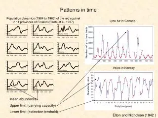
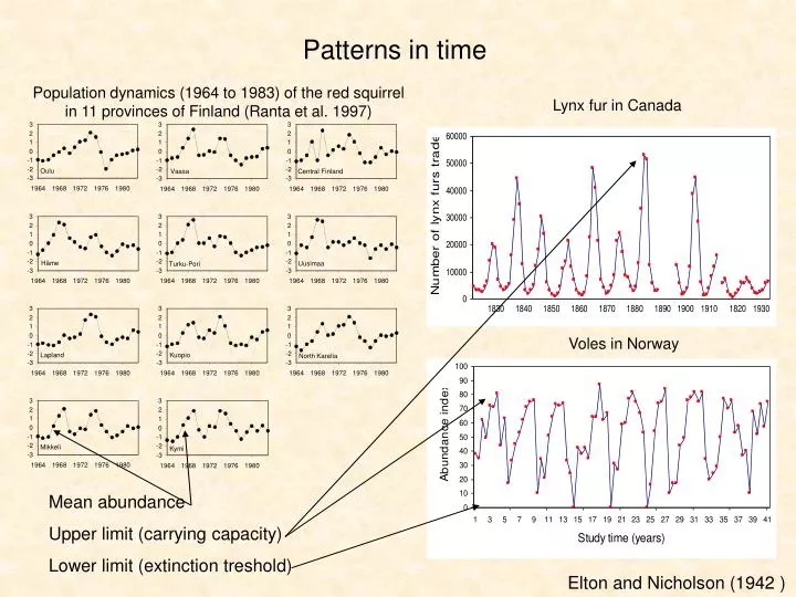
3 3 3 2 2 2 1 1 1 0 0 0 -1 -1 -1 -2 -2 -2 Oulu Vaasa Central Finland -3 -3 -3 1964 1968 1972 1976 1980 1964 1968 1972 1976 1980 1964 1968 1972 1976 1980 3 3 3 2 2 2 1 1 1 0 0 0 -1 -1 -1 -2 -2 -2 Häme Uusimaa Turku-Pori -3 -3 -3 1964 1968 1972 1976 1980 1964 1968 1972 1976 1980 1964 1968 1972 1976 1980 3 3 3 2 2 2 1 1 1 0 0 0 -1 -1 -1 -2 -2 -2 Lapland Kuopio North Karelia -3 -3 -3 1964 1968 1972 1976 1980 1964 1968 1972 1976 1980 1964 1968 1972 1976 1980 3 3 2 2 1 1 0 0 -1 -1 -2 -2 Mikkeli Kymi -3 -3 1964 1968 1972 1976 1980 1964 1968 1972 1976 1980 Patterns in time Population dynamics (1964 to 1983) of the red squirrel in 11 provinces of Finland (Ranta et al. 1997) Lynx fur in Canada Voles in Norway Mean abundance Upper limit (carrying capacity) Lower limit (extinction treshold) Elton and Nicholson (1942 )
Taylor’s power law Assume an assemblage of species, which have different mean abundances and fluctuate at random but proportional to their abundance. Going Excel The relationship between variance and mean follows a power function of the form Taylor’s power law; proportional rescaling
0.35 0.3 0.25 0.2 Percentage 0.15 0.1 0.05 0 0.2 0.6 1 1.4 1.8 2.2 2.6 3 3.4 Variance category Taylor’s power law Taylor’s power law in aphids (red), moths (green) and birds (blue). In all three groups the exponent z of the relation s2 = a mz peakes around 2. Data from Taylor et al. (1980).
Long term studies of population variability Major results from this database are that The variance – mean relationship of most populations follows Taylors power law z = 2 is equivalent to a random walk Z =<< 2 is required for population regulation The majority of species has 1.5 < z < 2.5 Most populations, in particular invertebrate populations are not regulated! They are not in equilibrium
Ecological implications Temporal variability is a random walk in time Abundances are not regulated Extinctions are frequent Temporal species turnover is high Temporal variability is intermediate Abundances are or are not regulated Extinctions are less frequent Temporal species turnover is low Temporal variability is low Abundances are often regulated Extinctions are rare Temporal species turnover is very low
Under theassumption of Taylor’spower law (a simple random walk in time withoutdensity dependent populationregulation and lowerextinctionboundary) we cancalculatethefrequency of localextinction Mean time to extinction Extinction probability
0.5 0.4 1 0.3 0.8 Normalized number of extinctions 0.2 0.6 Extinction probability 0.1 0.4 0 0.2 1 2 4 8 16 32 64 128 256 512 0.8 0 0.4 4 Number if individuals 6 8 10 0.1 12 15 20 Emigration 25 30 Number of patches rate 1 5 y = 0.06 / x y = 0.96x + 0.55 0.8 4 2 R = 0.46 0.6 3 ln (extinction time) Extinction probability 0.4 2 0.2 1 0 0 0 0.2 0.4 0.6 0.8 1 1.2 0 0.5 1 1.5 2 2.5 Mean number of nesting pairs ln (number of nesting pairs) How many individuals do populationsneed to survive(lowerextinctionboundary)? Orb web spiders on the Bahama islands (Schoener 1983) Parasitic Hymenoptera (Hassell et al. 1991) Birds on small islands off the British coast (Pimm 1991)
700 600 1.4 A B C 600 1.3 500 1.2 500 400 1.1 400 Turnover Number of species Number of species 300 300 1 200 200 0.9 100 0.8 100 0.7 0 0 0 5 10 0 50 100 150 0 50 100 150 Area Area t The species – time relationship Local species area and species time relationships in a temperate Hymenoptera community studied over a period of eight years. S = S0Az S = S0tt S = S0Aztt The accumulation of species richness in space and time follws a power function model Coeloides pissodis (Braconidae) Photo E. G. Vallery S = (73.0 ± 1.7)A(0.41 ± 0.01) t(0.094 ± 0.01) The mean extinction probability per year is about 9%
3 3 3 2 2 2 1 1 1 0 0 0 -1 -1 -1 -2 -2 -2 Oulu Vaasa Central Finland -3 -3 -3 1964 1968 1972 1976 1980 1964 1968 1972 1976 1980 1964 1968 1972 1976 1980 3 3 3 2 2 2 1 1 1 0 0 0 -1 -1 -1 -2 -2 -2 Häme Uusimaa Turku-Pori -3 -3 -3 1964 1968 1972 1976 1980 1964 1968 1972 1976 1980 1964 1968 1972 1976 1980 3 3 3 2 2 2 1 1 1 0 0 0 -1 -1 -1 -2 -2 -2 Lapland Kuopio North Karelia -3 -3 -3 1964 1968 1972 1976 1980 1964 1968 1972 1976 1980 1964 1968 1972 1976 1980 3 3 2 2 1 1 0 0 -1 -1 -2 -2 Mikkeli Kymi -3 -3 1964 1968 1972 1976 1980 1964 1968 1972 1976 1980 The Moran effect Regional sychronization of local abundances due to correlated environmental effects Population dynamics (1964 to 1983) of the red squirrel in 11 provinces of Finland Patrick A.P. Moran 1917-1988 Moran assumed: 1. Linear density dependence 2. Density dynamics are identical 3. Stochastic effects are correlated
20 30 40 50 60 70 80 90 Defoliation by gypsy moths in New England states 700000 Maine 600000 500000 Acres Defoliated 400000 300000 200000 100000 0 2500000 New Hampshire 2000000 1500000 Acres Defoliated 1000000 500000 0 140000 120000 Vermont 100000 Lymantria dispar Acres Defoliated 80000 60000 40000 20000 0 3000000 Massachusetts 2500000 2000000 Acres Defoliated 1500000 1000000 500000 0 Year Data from Williams and Liebhold (1995)
1.E+04 Protozoa Sessile marine organisms 1.E+03 1.E+02 Arthropoda Turnover rate (%/yr) 1.E+01 Birds 1.E+00 Lizards Vascular plants 1.E-01 1.E-04 1.E-03 1.E-02 1.E-01 1.E+00 1.E+01 1.E+02 1.E+03 25 25 Generation time 20 20 Body weight 15 15 Number of species Number of species 10 10 5 5 0 0 8000 6000 4000 2000 0 1977 1982 1987 1992 1997 Year Year 60 140 120 50 100 40 80 Number of species 30 Number of species 60 20 40 10 20 0 0 12000 9000 6000 3000 0 1940 1950 1960 1970 1980 1990 2000 Year Year Speciesturnoverrates (Brown et al. 2001) Species turnover rates differ between groups of animals and plants Larger animal species have lower turnover rates Desert rodents Plants Despite high turnover rates total species numbers of habitats remain largely constant. This constancy holds for ecological, historical and evolutionary times Birds Plants
Speciation rates, latitudinal gradients, and macroecology What causes the latitudinal gradient in species diversity? Temperature How does temperature influences species richness? Speciation Extinction Metabolic theory predicts that generation time t should scale to body weight and temperature to How does mean generation time decreases if we increase mean environmental temperature from 5º to 30 º? The theory predicts further that mutation rate a should scale to body weight and temperature to Mutation rates are predicted to increase by the same factor Evolutionary speed can be seen as the product of mutation rates and generation turnover (1/t). Still unclear is how temperature influences extinction rates.
Today’s reading Minimum viable population size: http://en.wikipedia.org/wiki/Minimum_viable_population Long term ecological research: http://www.lternet.edu/ Kinetic effects of temperature on speciation: http://www.pnas.org/content/103/24/9130.full.pdf Paleobiology: http://findarticles.com/p/articles/mi_m2120/is_n5_v77/ai_18601045