Slide Note
0 likes | 17 Views
Aggregate expenditure is the total value of finished goods and services in an economy, determined by consumption, planned investment, government spending, and net exports. Discrepancies between actual and planned investment can lead to changes in inventories. Equilibrium is achieved when Aggregate Expenditure equals GDP. Components of Aggregate Expenditure include consumption, planned investment, government purchases, and net exports. The relationship between income and consumption, as well as factors influencing planned investment, are crucial in understanding macroeconomic equilibrium.

E N D
Principles of Macroeconomics CHAPTER 8: AGGREGATE EXPENDITURE Unless otherwise noted, this work is licensed under a Creative Commons Attribution-NonCommercial-ShareAlike 4.0 International (CC BY-NC-SA 4.0) license. Feel free to use, modify, reuse or redistribute any portion of this presentation.
Learning Outcomes At the end of this chapter, you will be able to: Explain the Aggregate Expenditure Model Determine the Level of Aggregate Expenditure in the Economy Define Macroeconomic Equilibrium Identify the Multiplier Effect ● ● ● ●
8.0 Introduction The Great Recession of 2008- 2009 affected the Canadian economy The financial market meltdown called for action by the Federal Government ● ● Question: What caused this recession and what prevented the economy from spiraling further into recession?
8.1 Defining Aggregate Expenditure Aggregate expenditure is the current value of all the finished goods and services in the economy. ● The aggregate expenditure equation is: ● AE = C + I + G + NX Consumption (C): The household consumption over a period of time. Planned investment (I): Planned Planned spending on capital goods. Government expenditure (G): The amount of spending by federal, provincial, and local governments. Government expenditure can include infrastructure or transfers which increase the total expenditure in the economy. Net exports (NX): Total exports minus the total imports. ○ ○ ○ ○
8.1 Actual vs Planned Investment I When a company decides on how much to spend on investment, we assume they are deciding about business fixed expenditures. • The difference between actual investment and planned investment will be caused by an unexpected change in inventories. When actual investment spending exceeds planned investment spending, we see an unexpected increase in inventories. When actual investment spending is less than planned investment spending, we see an unexpected decrease in inventories. • o o
8.1 Actual vs Planned Investment II Let us assume Toyota manufactures 20,000 pick-up trucks in 2023, so planned investment would be based on the number of trucks manufactured. ● Suppose, Toyota was able to sell only 18,000 trucks by the end of the year, then actual investment would depend on the number of trucks sold. ● Due to changing economic circumstances, planned investment and actual investments may differ. ● Sometimes, businesses sell less due to falling consumer demand and therefore, actual investments would fall below planned. Whenever businesses can sell more due to growing demand, actual investments increase beyond planned. When Toyota manufactures 20K trucks, but sells only 18K, inventories build up, production and real GDP decrease. When Toyota manufactures 20K trucks, but sells 22K, inventories decrease, production and real GDP increase.
8.1 Equilibrium ● A macroeconomy is in equilibrium when Aggregate Expenditure = GDP
8.2 Components of AE: Consumption I Income can be consumed or saved. The relationship between income and consumption is called the consumption function. Consumption has an Autonomous part and an Induced part. Autonomous consumption does not depend on disposable income, induced part varies with disposable income. ●
8.2 Components of AE: Consumption II Because consumption heavily depends on income, we have a concept in the AE model called marginal propensity to consume (MPC). ● MPC = Change in Consumption ÷ ÷ Change in Disposable Income ● Marginal propensity to consume (MPC) is the share or percentage of additional income a person decides to consume (spend). ● Marginal propensity to save (MPS) is the share of additional income a person decides to save. ● MPC + MPS = 1 must always hold true since the only options are to consume or save income.
8.2 Components of AE: Consumption III The relationship between income and consumption can be extended to the national economy as any increase in national income will lead to an increase in consumption. National Income = GDP = Disposable income + Net taxes
8.2 Components of AE: Planned Investment I Planned investment is determined by: Expectations of future profitability The real interest rate Taxes Cash flow ● ○ ○ ○ ○
8.2 Components of AE: Planned Investment II The investment function shows the relationship between real GDP and investment levels. The investment function can be drawn as a horizontal line as investment decisions do not depend primarily on the level of GDP in the current year. Investment is called an Autonomous expenditure, that does not depend on real GDP. ● ●
8.2 Components of AE: Government Purchases Federal, provincial, and local governments determine the level of government spending. Government spending is independent of GDP and so is shown as a horizontal line. ● ● Government spending is called an Autonomous expenditure, that does not depend on real GDP. ●
8.2 Components of AE: Net Exports Exports do not depend on a country's national income (GDP), so exports are autonomous too. ● The import function is connected to national income. As income grows, a country’s ability to import increases. The slope of the function (line) = marginal propensity to import (MPI) where the percentage change in spending on imports when national income changes. ● ○
8.3 The Aggregate Expenditure Function I The aggregate expenditure function shows the total expenditures in the economy for each level of real GDP. To find the aggregate expenditure function sum the parts using the equation C + I + G + (X-M) = AE The equilibrium level of AE is $6000 in the table below where AE = GDP ● ● ●
8.3 The Aggregate Expenditure Function II Graphically, the aggregate expenditure function is formed by stacking: the consumption function the investment function the government spending function the net export function ● ○ ○ ○ ○
8.3 The Aggregate Expenditure Function III Point E0is the equilibrium for the economy This point is where total amount being spend equals the total level of production ● ●
8.3 The Aggregate Expenditure Function IV The point of intersection between the aggregate expenditure function and the 45° line is a macroeconomic equilibrium. No change in inventories. To the right of equilibrium (i.e. at H) output is higher than AE, spending falls and unsold inventories pile up. To the left of equilibrium (i.e. at L) output is lower than AE, spending increases and store shelves get empty, inventories decline. ● ● ●
8.4 The Multiplier I Changes in any category of expenditure have a more than proportional impact on GDP. The multiplier shows that the change in GDP is a multiple of the change in any autonomous expenditure (I, G or X) ● ○ Changes in autonomous variables cause the AE curve to shift vertically creating a new equilibrium. ●
8.4 The Multiplier II In this example there is an increase in Government expenditure Original increase in aggregate expenditure from government purchase 100 Second round of increase in AE from additional consumption... 100+80 = 180 Third-round increase in AE due to induced consumption from additional income in second round 180 + 60 = 240 Fourth round increase in AE due to further induced consumption from additional expenditure incurred in round 3 240 + 40 = 280
8.4 The Multiplier III First formula for calculating the multiplier: ● Multiplier = 1 ÷ ÷ (1- MPC) When MPC = 0.8, multiplier = 1/(1 – 0.8) = 5 implying, a dollar increase in G, increases GDP by $5. Second formula for calculating the multiplier: ● Change in GDP ÷ ÷ change in any autonomous expenditure (I, G, or X) When a G increase by $100M increases GDP by $500M, multiplier = $500M/$100M = 5 The multiplier applies when expenditure decreases as well as when it increases. ●
8.5 Key Terms Aggregate expenditure Autonomous consumption Autonomous Expenditure Consumption Consumption function Induced expenditure Investment function Macroeconomy equilibrium Marginal propensity to consume (MPC) Marginal propensity to import (MPI) Marginal propensity to save (MPS) Multiplier Wealth ● ● ● ● ● ● ● ● ● ● ● ● ●