Download
1 / 18
180 likes | 297 Views
>> n=-50:50; wc=0.4*pi; >> hn=sinc(n*wc/pi)*wc/pi; >> stem(n,hn); title('Ideal LPF with cutoff frequency = 0.4 pi'). >> w=linspace(0,pi,512); mag_hw= cos (w/2); >> [h,w1]=freqz([0.5 0.5],[1]); >> subplot(2,1,1); plot(w/pi,mag_hw);title('|H(omega)|of first order FIR LPF:analytical solution')

E N D
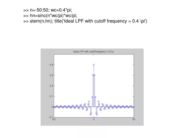
>> n=-50:50; wc=0.4*pi; >> hn=sinc(n*wc/pi)*wc/pi; >> stem(n,hn); title('Ideal LPF with cutoff frequency = 0.4 \pi')
>> w=linspace(0,pi,512); mag_hw=cos(w/2); >> [h,w1]=freqz([0.5 0.5],[1]); >> subplot(2,1,1); plot(w/pi,mag_hw);title('|H(\omega)|of first order FIR LPF:analytical solution') >> subplot(2,1,2); plot(w1/pi,abs(h));title('|H(\omega)|of first order FIR LPF:FREQZ')
>> w=linspace(0,pi,512); mag_hw=sin(w/2); >> [h,w1]=freqz([0.5 -0.5],[1]); >> subplot(2,1,1); plot(w/pi,mag_hw);title('|H(\omega)|of first order FIR HPF:analytical solution') >> subplot(2,1,2); plot(w1/pi,abs(h));title('|H(\omega)|of first order FIR HPF:FREQZ')
>> w=linspace(0,pi,512); mag_hw=abs(sinc(w*(M+1)/2/pi)./sinc(w/2/pi)); >> b=ones(1,M+1)/(M+1);a=[1]; >> [h,w1]=freqz(b,a); >> subplot(2,1,1); plot(w/pi,mag_hw);title('|H(\omega)|of moving average filter (M=10):analytical solution') >> subplot(2,1,2); plot(w1/pi,abs(h));title('|H(\omega)|of moving average filter (M=10):FREQZ')
>> b=[5,2];a=[1, -0.8]; >> freqz(b,a)
>> freqz(b,a) >> b=[5 -0.4];a=[1 0.4]; >> zplane(b,a)
>> b=[0.15,0,-0.15]; a=[1,0,0.7]; >> zplane(b,a) >> freqz(b,a)
>> b=poly([0.9*exp(j*pi/2) 0.9*exp(-j*pi/2)]) b = 1.0000 -0.0000 0.8100 >> a=poly([0.8 -0.8]) a = 1.0000 0 -0.6400 >> zplane(b,a) >> freqz(b,a)
>> R=0.9;w0=pi/3; >> a1=-2*R*cos(w0);a2=R^2; >> G=(1-R)*sqrt(1-2*R*cos(2*w0)+R^2); >> b=[G]; a=[1 a1 a2]; >>zplane(b,a) >> freqz(b,a)
>> R=0.8;r=0.7;w0=pi/3; >> a1=-2*R*cos(w0);a2=R^2; >> b1=-2*r*cos(w0);b2=r^2; >> b=[1 b1 b2];a=[1 a1 a2]; >> zplane(b,a) >> freqz(b,a)
>> R=0.8;r=0.785;w0=pi/3; >> a1=-2*R*cos(w0);a2=R^2; >> b1=-2*r*cos(w0);b2=r^2; >> b=[1 b1 b2];a=[1 a1 a2]; >> zplane(b,a) >> freqz(b,a)
>> R=0.8;r=0.815;w0=pi/3; >> a1=-2*R*cos(w0);a2=R^2; >> b1=-2*r*cos(w0);b2=r^2; >> b=[1 b1 b2];a=[1 a1 a2]; >> zplane(b,a) >> freqz(b,a)
>> R=0.98;r=1;w0=pi/3; >> a1=-2*R*cos(w0);a2=R^2; >> b1=-2*r*cos(w0);b2=r^2; >> b=[1 b1 b2];a=[1 a1 a2]; >> zplane(b,a) >> freqz(b,a)