Download
1 / 72
740 likes | 983 Views
ESSENTIAL CALCULUS CH04 Integrals. In this Chapter:. 4.1 Areas and Distances 4.2 The Definite Integral 4.3 Evaluating Definite Integrals 4.4 The Fundamental Theorem of Calculus 4.5 The Substitution Rule Review. Chapter 4, 4.1, P194. Chapter 4, 4.1, P195. Chapter 4, 4.1, P195.

E N D
In this Chapter: • 4.1 Areas and Distances • 4.2 The Definite Integral • 4.3 Evaluating Definite Integrals • 4.4 The Fundamental Theorem of Calculus • 4.5 The Substitution Rule Review
2. DEFINITION The area A of the region S that lies under the graph of the continuous function f is the limit of the sum of the areas of approximating rectangles: A=lim Rn=lim[f(x1)∆x+f(x2) ∆x+‧‧‧+f(xn) ∆x] n→∞ n→∞ Chapter 4, 4.1, P199
This tells us to end with i=n. This tells us to add. This tells us to start with i=m. Chapter 4, 4.1, P199
The area of A of the region S under the graphs of the continuous function f is A=lim[f(x1)∆x+f(x2) ∆x+‧‧‧+f(xn) ∆x] A=lim[f(x0)∆x+f(x1) ∆x+‧‧‧+f(xn-1) ∆x] A=lim[f(x*1)∆x+f(x*2) ∆x+‧‧‧+f(x*n) ∆x] n→∞ n→∞ n→∞ Chapter 4, 4.1, P200
FIGURE 1 A partition of [a,b] with sample points Chapter 4, 4.2, P205
A Riemann sum associated with a partition P and a function f is constructed by evaluating f at the sample points, multiplying by the lengths of the corresponding subintervals, and adding: Chapter 4, 4.2, P205
FIGURE 2 A Riemann sum is the sum of the areas of the rectangles above the x-axis and the negatives of the areas of the rectangles below the x-axis. Chapter 4, 4.2, P206
2. DEFINITION OF A DEFINITE INTEGRAL If f is a function defined on [a,b] ,the definite integral of f from a to b is the number provided that this limit exists. If it does exist, we say that f is integrable on [a,b] . Chapter 4, 4.2, P206
NOTE 1 The symbol ∫was introduced by Leibniz and is called an integral sign. It is an elongated S and was chosen because an integral is a limit of sums. In the notation is called the integrand and a and b are called the limits of integration; a is the lower limit and b is the upper limit. The symbol dx has no official meaning by itself; is all one symbol. The procedure of calculating an integral is called integration. Chapter 4, 4.2, P206
3. THEOREM If f is continuous on [a,b], or if f has only a finite number of jump discontinuities, then f is integrable on [a,b]; that is, the definite integral dx exists. Chapter 4, 4.2, P207
4. THEOREM If f is integrable on [a,b], then where Chapter 4, 4.2, P207
MIDPOINT RULE where and Chapter 4, 4.2, P211
PROPERTIES OF THE INTEGRAL Suppose all the following integrals exist. where c is any constant where c is any constant Chapter 4, 4.2, P213
COMPARISON PROPERTIES OF THE INTEGRAL 6. If f(x)≥0 fpr a≤x≤b. then 7.If f(x)≥g(x) for a≤x≤b, then 8.If m≤f(x) ≤M for a≤x≤b, then Chapter 4, 4.2, P214
29.The graph of f is shown. Evaluate each integral by interpreting it in terms of areas. • (b) • (c) (d) Chapter 4, 4.3, P217
30. The graph of g consists of two straight lines and a semicircle. Use it to evaluate each integral. (a) (b) (c) Chapter 4, 4.3, P217
EVALUATION THEOREM If f is continuous on the interval [a,b] , then Where F is any antiderivative of f, that is, F’=f. Chapter 4, 4.3, P218
the notation ∫f(x)dx is traditionally used for an antiderivative of f and is called an indefinite integral. Thus The connection between them is given by the Evaluation Theorem: If f is continuous on [a,b], then Chapter 4, 4.3, P220
▓You should distinguish carefully between definite and indefinite integrals. A definite integral is a number, whereas an indefinite integral is a function (or family of functions). Chapter 4, 4.3, P220
1. TABLE OF INDEFINITE INTEGRALS Chapter 4, 4.3, P220
■ Figure 3 shows the graph of the integrand in Example 5. We know from Section 4.2 that the value of the integral can be interpreted as the sum of the areas labeled with a plus sign minus the area labeled with a minus sign. Chapter 4, 4.3, P221