
Linear Regression with One Predictor Variable
E N D
Presentation Transcript
Linear Regression with One Predictor Variable Ayona Chatterjee Spring 2008 Math 4803/5803
Introduction • Statistical methodology that utilizes the relationship between two quantitative variables. • Use explanatory variables (independent, X) to predict the outcome/response (dependent, Y). • Introduced by Sir Francis Galton while studying heights of offspring and parents.
Examples • Sales of a product can be predicted by utilizing the relationship between sales and amount of advertising expenditures. • Performance of a student in a test can be predicted using the students IQ and time spent studying. • Length of a hospital stay of a surgical patient can be predicted by using the relationship between the time in the hospital and the severity of the operation.
Types of Relations between Variables • Functional Relationship • A functional relationship between two variables is expressed by a mathematical formula. If X denotes the independent variable and Y denotes the dependent variable, a functional relation is of the form Y = f(X). • Statistical Relationship • Unlike a functional relation, does not lie on a straight lie. There is scope for some error.
Example of Statistical Relation • Performance of 10 students were obtained at mid-semester and at end of semester for a statistics exam. The data are plotted in the next slide. The end of semester grades are taken as dependent (Y) and the mid term grades are assumed to be the explanatory variable (X).
Basic Concept • A tendency of the response variable Y to vary with the predictor variable X in a systematic fashion. • There is a probability distribution of Y for each level of X. • A scattering of points around the curve of statistical relationship. • The means of these distributions vary in some systematic fashion with X.
Note • A regression model can be linear or curvilinear. • A regression model can have more than one predictor variable. • We will look at multiple regression later on.
Construction of Regression Models • Selection of Predictor Variables. • Construct models with limited number of explanatory variables to have a practical model. • Choose variables that help in reducing variation in Y. • Functional Form of Regression Relation. • Depends on the explanatory variable. • May be available from existing literature. • Or else it has to be decided empirically once the data are collected.
Construction of Regression Models • Scope of Model. • The regression equation is only valid in the range of data used to obtain it. • Uses of Regression Analysis • Description • Control • Prediction
Regression and Causality • No cause-and-effect pattern is necessarily implied by the regression model. • Regression analysis by itself provides no information about causal patterns and must be supplemented by additional analyses. • Example:Data on size of vocabulary (X) and writing speed (Y) for a sample of children aged 5-10 will show a positive regression relation. This does not imply that an increase in vocabulary causes faster writing speed.
Simple Linear Regression Model • With only one predictor, the model is as follows: • Where • Yi is the value of the response variable in the ith trail. • β0 and β1 are parameters • Xi us a known constant, value of the predictor variable in the ith trail. • εi is the random error term with mean 0, variance σ2 and covariance zero. • i= 1………n
Meaning of Regression Parameters • The parameters β0 and β1 are called regression coefficients. • Here β1 is the slope of the regression line and indicates the change in the mea of the probability distribution of Y per unit increase in X. • When sensible, β0 is the mean of the probability distribution for Y when X =0.
Example • A consultant for an electrical distributor is studying the relationship between the number of bids requested by construction contractor for basic lighting equipment during a week and the time required to prepare the bids. Let X be the number of bids prepared in a week and Y is the number of hours required to prepare the bids. • Suppose the regression function is: • Y = 9.5 + 2.1 X + ε • Here slope 2.1 indicates the preparation of one additional bid in a week leads to an increase in the mean of the probability distribution of Y of 2.1 hours. • Here X=0 is of no practical use so β0has no particular meaning.
Data for Regression Analysis • Observational Data • Obtained from non-experimental studies. • Experimental Data • Completely Randomized Data (CRD) • All combinations of experimental unit has an equal chance to receive any one of the treatments. • For all our studies we shall you CRD.
Estimation of Regression Function • We will use the method of Least squares to obtain estimates for β0 and β1. • Lets do it by hand! • The Gauss-Markov theorem gives us that b0 and b1 are unbiased and have minimum variance among all unbiased linear estimator.
Residuals • The ith residual is the difference between the observed value Yi and the corresponding fitted value. This residual is denoted by ei an is defined in general as follows: • Where the fitted value is given by • Remember residuals are known where as the error term εi from the model is unknown.
Some Properties of Fitted Regression Line • Sum of residual is zero: • The sum of the squared residuals is minimum. • Sum of the observed values equal the sum of the fitted values. • The regression line always goes through .
Estimation of Error Terms Variance • The mean square error (MSE) is used to estimate the error variance of the data s2. • MSE is an unbiased estimate for σ2. • Here
Normal Error Regression Model • This is the same model as described before only the with additional assumption that the error term εi is Normally distributed with mean 0 and variance σ2. • For all our regression models we will assume normal error terms.
Practice Problem • Look at the data sheet given to you and answer the questions.