
Single Queue Modeling for System Performance Predictions
E N D
Presentation Transcript
Basic definitions for performance predictions The performance of a system that gives services could be seen from two different viewpoints: • user: the time to obtain a service or the waiting time before getting a service; • system: the number of users served in the unit time or the resources utilization level.
Basic definitions for performance predictions The model can be built analyzing the behaviour of the system.
Arrival rate and throughput Principal measures: • T: system observation interval; • A: number of arrivals in the period T; • C: number of completions in the period T. Derived quantities: • λ: arrival rate, λ = A/T; • X: throughput, X= C/T.
Utilization factor For a single server an interesting measure is also the period the server is busy (B). Then we can obtain: • ρ:server utilization, ρ =B/T; • S: average service completion per request, B/C. Now it is possible to get the utilization law: ρ= B/T = S C/T = X S a special case of the Little’s law
Little’s law Denoting with: • W : the time spent in system by the all requests in T • N: the average number of requests in the system, N = W/T • R: the average system residence time per request (average response time), R=W/C the Little’s law is equal to: N=X R given that N = W/T= R C/T Little’s law is very important in the performance evaluation of system consisting of a set of servers because it is widely applicable and does not require strong assumptions.
Queuing systems A system can be modelled by a set of interconnected queues. The servers and the users have different characteristics/behaviorsin each queue. If the queues have an independent each other behaviour, then each queue can be analysed separately. In particular conditions each queue can be modelled as a Markov chain.
Queuing systems For example a birth/dead process can be used to represent a particular queue in which: • the inter arrival time of the users is distributed in accordance to the exponential distribution, with arrival rate equal to λ; • the presence of only one server; • the service time is distributed in accordance to the exponential distribution, with service time equal to 1/μ. This kind of queue is denoted as M/M/1
l l l l . . . . 1 2 0 3 m m m m M/M/1 queue analysis Infinite queue State transition diagram – infinite population
l l l l . . . . 1 0 2 3 m m m m M/M/1 queue analysis Infinite queue State transition diagram with boundaries
M/M/1 queue analysis At every state, in a balanced condition the incoming flow is equal to the outgoing flow.
M/M/1 queue analysis Solving the system: The sum of the time fractions the system being in all possible states, from 0 to ∞, equals to 1 (probability):
M/M/1 queue analysis we obtain ↓
M/M/1 queue analysis It is now possible to calculate the following quantities: Probability to stay in state k (fraction of time server has k requests): where then
M/M/1 queue analysis The utilization factor: The expected number of users in the system Using the “average” definition, The last sum is equals to U/(1-U)2for U<1,
M/M/1 queue analysis The average response time Using the Little’s Law (the average throughput equals to ), where S=1/ is the average service time of request at the server. The expected number of users in the queue The average time in the queue and in the system
Example (infinite queue) Arrival rate at the Web server: =30 requests/sec Average service time: 0.02 seconds Solution Average service rate → = 1/0.02 = 50 request/sec U=/ → U=30/50=0.6 (60%) p0=1-U=1-0.6=40% Average number of requests at the server: N=U/(1-U)=0.6/(1-0.6)=1.5 Average response time: R=S/(1-U)=(1/ )/(1-U)=(1/50)/(1-0.6)=0.05sec
l l l l l l . . . . . . . W 1 2 0 K 3 m m m m m m M/M/1 finite queue analysis Finite queue State transition diagram – infinite population/finite queue
M/M/1 finite queue analysis Using the flow-in=flow-out equations, We have a finite number of states,
M/M/1 finite queue analysis Hence, The utilization factor: U=1-p0 →
M/M/1 finite queue analysis The expected number of users in the system Using the “average” definition:
M/M/1 finite queue analysis The average response time Using the Little’s Law and S=1/ :
Example (finite queue) Arrival rate at the Web server: =30 requests/sec Average service time: 0.02 seconds Minimum queue length so that less than 1% of requests are rejected Solution Average service rate → = 1/0.02 = 50 request/sec U=/ → U=30/50=0.6 (60%) p0=0.4/(1-0.6W+1) pW=p0(/)W<0.01 → 0.4* 0.6W/(1-0.6W+1)<0.01 → W≥8
l0 l1 l2 k-1 lk . . . . 1 2 0 k m1 m3 mk+1 m2 mk Generalized System-Level Models Using the flow-in=flow-out equations,
Generalized System-Level Models By applying recursively,
Generalized System-Level Models So, Since
Generalized System-Level Models this implies that