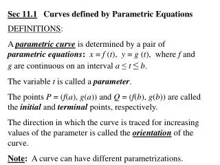
Plane Curves and Parametric Equations
300 likes | 765 Views
Plane Curves and Parametric Equations. New Ways to Describe Curves (10.4). POD. Describe this curve. Is it a function?. POD. Describe this curve. A circle with center at (-2, 3), and radius 11. Is it a function? Nope. New vocabulary.

Plane Curves and Parametric Equations
E N D
Presentation Transcript
Plane Curves and Parametric Equations New Ways to Describe Curves (10.4)
POD Describe this curve. Is it a function?
POD Describe this curve. A circle with center at (-2, 3), and radius 11. Is it a function? Nope.
New vocabulary y = f(x) is a function, if f is a function. We know how this works. This is an example of a plane curve, but plane curves also include non-functions, like the conics we’ve been studying.
New vocabulary Various examples P(a) and P(b) are the endpoints of curve C. If P(a) = P(b), the curve is a closed curve. If there is not overlap, it is a simple closed curve. Is there a way to describe these non-functions in terms of functions? (Of course there is, or we wouldn’t be doing this.) P(a) P(a) = P(b) P(b)
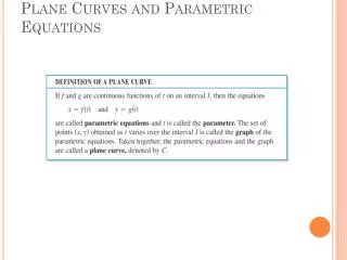
New vocabulary Plane curve: a set C of ordered pairs (f(t),g(t)), where f and g are functions defined on interval I. In other words, a graph may not be a function, but we substitute the coordinates x and y with separate components that are functions of t– a mathematical sleight of hand. Then we specify an interval I to run t in.
Parametric equations We use parametric equations to describe plane curves. The format is a bit different from the y = form we’re used to– we add a third variable and base the x and y functions on it. The curve C with parameter t: x = f(t) y = g(t) for t in interval I. The final result is a curve– which could be the same as curves we’ve seen– which runs in a particular direction (orientation).
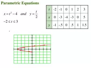
Parametric equations– use it The curve C with parameter t: x = f(t) y = g(t) for t in I. 1. x = 2t y = t2 -1 -1 ≤ t ≤ 2 a. On calculators, graph the curve, and determine its orientation. Change the T window and T step to see how the graph changes. b. Do this with a triple-column chart on the next slide. c. Combine them to find an equation in x and y (a more familiar form).
Parametric equations– use it 1. x = 2t y = t2 -1 -1 ≤ t ≤ 2 a. Graph the curve, and show its orientation. We can do this easily on the graphing calculators. Change the MODE to “PARA” for parametric mode. The Y= window is different, and we include both functions.
Parametric equations– use it 1. x = 2t y = t2 -1 -1 ≤ t ≤ 2 a. Plot the curve, and show its orientation. The window screen is also different– we include the final x and y dimensions, of course, but add the interval and increments for t.
Parametric equations– use it 1. x = 2t y = t2 -1 -1 ≤ t ≤ 2 a. Plot the curve, and show its orientation. The final graph looks like something we’ve seen before. Why does it stop?
Parametric equations– use it 1. x = 2t y = t2 -1 -1 ≤ t ≤ 2 b. Plot the curve, and show its orientation. t x y -1 -½ 0 ½ 1 3/2 2 It’s like there are two dependent variables (x and y) based on one independent variable (t). How does the curve “run”?
Parametric equations– use it 1. x = 2t y = t2 -1 -1 ≤ t ≤ 2 c. Combine them to find an equation in x and y (a more familiar form). x = 2t t = x/2 y = t2 -1 y = (x/2)2 -1 y= ¼ x2 -1
Parametric equations– use it 1. x = 2t y = t2 -1 -1 ≤ t ≤ 2 One curve can be expressed by an infinite number of parametric equations. x = t y = ¼ t2 – 1 -2 ≤ t ≤ 4 x = t3 y = (1/8) t6 – 1 -21/3 ≤ t ≤ 41/3 Try graphing them on calculators.
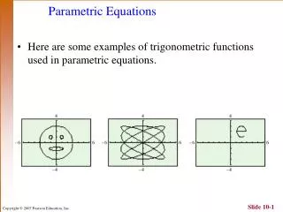
Parametric equations– use it 2. P(x, y) is x = a cos t and y = a sin t, for all real number values of t, and a >0. Describe the motion of P. Don’t graph, just think.
Parametric equations– use it 2. P(x, y) is x = a cos t and y = a sin t, for all real number values of t, and a >0. Describe the motion of P. Don’t graph, just think. Graph on calculators. Set a = 5.
Parametric equations– use it 2. P(x, y) is x = a cos t and y = a sin t, for all real number values of t, and a >0. Describe the motion of P.
Parametric equations– use it 2. P(x, y) is x = a cos t and y = a sin t, for all real number values of t, and a >0. Describe the motion of P. Why look, a circle with radius a, centered on the origin. The curve follows a counter-clockwise rotation. Graph it on calculators to check. Radian or degree mode?
Parametric equations– use it 3. From p. 824, #4. Graph the parametric equation and give its orientation. What is the equation in x-y notation? x = t3 + 1 y = t3 – 1 -2 ≤ t ≤ 2
Parametric equations– use it 3. From p. 824, #4. Graph the parametric equation and give its orientation. What is the equation in x-y notation? x = t3 + 1 y = t3 – 1 -2 ≤ t ≤ 2 What does this curve look like?
Parametric equations– use it 3. From p. 824, #4. Graph the parametric equation and give its orientation. What is the equation in x-y notation? x = t3 + 1 y = t3 – 1 -2 ≤ t ≤ 2 t x y -2 -1 0 1 2
Parametric equations– use it 3. From p. 824, #4. Graph the parametric equation and give its orientation. What is the equation in x-y notation? x = t3 + 1 y = t3 – 1 -2 ≤ t ≤ 2 t3 = x – 1 y = (x – 1) – 1 y = x – 2