Download
1 / 53
530 likes | 603 Views
Explore data prediction, confidence, and ILP limits in computer architecture lecture; review branch prediction and speculation, memory dependence prediction, and load value predictability techniques.

E N D
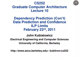
CS252Graduate Computer ArchitectureLecture 10Dependency Prediction (Con’t)Data Prediction and Confidence ILP LimitsFebruary 23rd, 2011 John Kubiatowicz Electrical Engineering and Computer Sciences University of California, Berkeley http://www.eecs.berkeley.edu/~kubitron/cs252
Branch Resolution kill kill kill kill Review: Branch Prediction/Speculation Update predictors Branch Prediction PC Fetch Decode & Rename Reorder Buffer Commit Reg. File MEM Branch Unit ALU Store Buffer D$ Execute CS252-S11 lecture 10
Review: Memory Disambiguation • Question: Given a load that follows a store in program order, are the two related? • Trying to detect RAW hazards through memory • Stores commit in order (ROB), so no WAR/WAW memory hazards. • Implementation • Keep queue of stores, in program order • Watch for position of new loads relative to existing stores • Typically, this is a different buffer than ROB! • Could be ROB (has right properties), but too expensive • When have address for load, check store queue: • If any store prior to load is waiting for its address????? • If load address matches earlier store address (associative lookup), then we have a memory-induced RAW hazard: • store value available return value • store value not available return ROB number of source • Otherwise, send out request to memory • Will relax exact dependency checking in later lecture CS252-S11 lecture 10
Memory Dependence Prediction • Important to speculate? Two Extremes: • Naïve Speculation: always let load go forward • No Speculation: always wait for dependencies to be resolved • Compare Naïve Speculation to No Speculation • False Dependency: wait when don’t have to • Order Violation: result of speculating incorrectly • Goal of prediction: • Avoid false dependencies and order violations • From “Memory Dependence Prediction • using Store Sets”, Chrysos and Emer. CS252-S11 lecture 10
Said another way: Could we do better? • Results from same paper: performance improvement with oracle predictor • We can get significantly better performance if we find a good predictor • Question: How to build a good predictor? CS252-S11 lecture 10
Premise: Past indicates Future • Basic Premise is that past dependencies indicate future dependencies • Not always true! Hopefully true most of time • Store Set: Set of store insts that affect given load • Example: Addr Inst 0 Store C 4 Store A 8 Store B 12 Store C 28 Load B Store set { PC 8 } 32 Load D Store set { (null) } 36 Load C Store set { PC 0, PC 12 } 40 Load B Store set { PC 8 } • Idea: Store set for load starts empty. If ever load go forward and this causes a violation, add offending store to load’s store set • Approach: For each indeterminate load: • If Store from Store set is in pipeline, stallElse let go forward • Does this work? CS252-S11 lecture 10
How well does an infinite tracking work? • “Infinite” here means to place no limits on: • Number of store sets • Number of stores in given set • Seems to do pretty well • Note: “Not Predicted” means load had empty store set • Only Applu and Xlisp seems to have false dependencies CS252-S11 lecture 10
How to track Store Sets in reality? • SSIT: Assigns Loads and Stores to Store Set ID (SSID) • Notice that this requires each store to be in only one store set! • LFST: Maps SSIDs to most recent fetched store • When Load is fetched, allows it to find most recent store in its store set that is executing (if any) allows stalling until store finished • When Store is fetched, allows it to wait for previous store in store set • Pretty much same type of ordering as enforced by ROB anyway • Transitivity loads end up waiting for all active stores in store set • What if store needs to be in two store sets? • Allow store sets to be merged together deterministically • Two loads, multiple stores get same SSID • Want periodic clearing of SSIT to avoid: • problems with aliasing across program • Out of control merging CS252-S11 lecture 10
How well does this do? • Comparison against Store Barrier Cache • Marks individual Stores as “tending to cause memory violations” • Not specific to particular loads…. • Problem with APPLU? • Analyzed in paper: has complex 3-level inner loop in which loads occasionally depend on stores • Forces overly conservative stalls (i.e. false dependencies) CS252-S11 lecture 10
Load Value Predictability • Try to predict the result of a load before going to memory • Paper: “Value locality and load value prediction” • Mikko H. Lipasti, Christopher B. Wilkerson and John Paul Shen • Notion of value locality • Fraction of instances of a given loadthat match last n different values • Is there any value locality in typical programs? • Yes! • With history depth of 1: most integerprograms show over 50% repetition • With history depth of 16: most integerprograms show over 80% repetition • Not everything does well: see cjpeg, swm256, and tomcatv • Locality varies by type: • Quite high for inst/data addresses • Reasonable for integer values • Not as high for FP values CS252-S11 lecture 10
Instruction Addr LVPT Prediction Results Load Value Prediction Table • Load Value Prediction Table (LVPT) • Untagged, Direct Mapped • Takes Instructions Predicted Data • Contains history of last n unique values from given instruction • Can contain aliases, since untagged • How to predict? • When n=1, easy • When n=16? Use Oracle • Is every load predictable? • No! Why not? • Must identify predictable loads somehow CS252-S11 lecture 10
LCT Predictable? Correction Load Classification Table (LCT) Instruction Addr • Load Classification Table (LCT) • Untagged, Direct Mapped • Takes Instructions Single bit of whether or not to predict • How to implement? • Uses saturating counters (2 or 1 bit) • When prediction correct, increment • When prediction incorrect, decrement • With 2 bit counter • 0,1 not predictable • 2 predictable • 3 constant (very predictable) • With 1 bit counter • 0 not predictable • 1 constant (very predictable) CS252-S11 lecture 10
Accuracy of LCT • Question of accuracy is about how well we avoid: • Predicting unpredictable load • Not predicting predictable loads • How well does this work? • Difference between “Simple” and “Limit”: history depth • Simple: depth 1 • Limit: depth 16 • Limit tends to classify more things as predictable (since this works more often) • Basic Principle: • Often works better to have one structure decide on the basic “predictability” of structure • Independent of prediction structure CS252-S11 lecture 10
Constant Value Unit • Idea: Identify a load instruction as “constant” • Can ignore cache lookup (no verification) • Must enforce by monitoring result of stores to remove “constant” status • How well does this work? • Seems to identify 6-18% of loads as constant • Must be unchanging enough to cause LCT to classify as constant CS252-S11 lecture 10
Load Value Architecture • LCT/LVPT in fetch stage • CVU in execute stage • Used to bypass cache entirely • (Know that result is good) • Results: Some speedups • 21264 seems to do better than Power PC • Authors think this is because of small first-level cache and in-order execution makes CVU more useful CS252-S11 lecture 10
Administrivia • Exam: Week after 3/16? • CS252 First Project proposal due by Friday 3/4 • Need two people/project (although can justify three for right project) • Complete Research project in 9 weeks • Typically investigate hypothesis by building an artifact and measuring it against a “base case” • Generate conference-length paper/give oral presentation • Often, can lead to an actual publication. CS252-S11 lecture 10
Timing Model Pipeline Functional Model Pipeline Arch State Timing State One important tool is RAMP Gold: FAST Emulation of new Hardware • RAMP emulation model for Parlab manycore • SPARC v8 ISA -> v9 • Considering ARM model • Single-socket manycore target • Split functional/timing model, both in hardware • Functional model: Executes ISA • Timing model: Capture pipeline timing detail (can be cycle accurate) • Host multithreading of both functional and timing models • Built for Virtex-5 systems (ML505 or BEE3) • Have Tessellation OS currently running on RAMP system! CS252-S11 lecture 10
Large Compute-Bound Application Firewall Virus Intrusion Monitor And Adapt Real-Time Application Video & Window Drivers Persistent Storage & File System HCI/ Voice Rec Device Drivers Identity Tessellation: The Exploded OS • Normal Components split into pieces • Device drivers (Security/Reliability) • Network Services (Performance) • TCP/IP stack • Firewall • Virus Checking • Intrusion Detection • Persistent Storage (Performance, Security, Reliability) • Monitoring services • Performance counters • Introspection • Identity/Environment services (Security) • Biometric, GPS, Possession Tracking • Applications Given Larger Partitions • Freedom to use resources arbitrarily CS252-S11 lecture 10
Space Time Space Space-Time Resource Graph Implementing the Space-Time Graph Partition Policy Layer (Resource Allocator) Reflects Global Goals • Partition Policy layer (allocation) • Allocates Resources to Cells based on Global policies • Produces only implementable space-time resource graphs • May deny resources to a cell that requests them (admission control) • Mapping layer (distribution) • Makes no decisions • Time-Slices at a course granularity (when time-slicing necessary) • performs bin-packing like operation to implement space-time graph • In limit of many processors, no time multiplexing processors, merely distributing resources • Partition Mechanism Layer • Implements hardware partitions and secure channels • Device Dependent: Makes use of more or less hardware support for QoS and Partitions Mapping Layer (Resource Distributer) Partition Mechanism Layer ParaVirtualized Hardware To Support Partitions CS252-S11 lecture 10
Sample of what could make good projects • Implement new resource partitioning mechanisms on RAMP and integrate into OS • You can actually develop a new hardware mechanism, put into the OS, and show how partitioning gives better performance or real-time behavior • You could develop new message-passing interfaces and do the same • Virtual I/O devices • RAMP-Gold runs in virtual time • Develop devices and methodology for investigating real-time behavior of these devices in Tessellation running on RAMP • Energy monitoring and adaptation • How to measure energy consumed by applications and adapt accordingly • Develop and evaluate new parallel communication model • Target for Multicore systems • New Message-Passing Interface, New Network Routing Layer • Investigate applications under different types of hardware • CUDA vs MultiCore, etc • New Style of computation, tweak on existing one • Better Memory System, etc. CS252-S11 lecture 10
Projects using Quantum CAD Flow • Use the quantum CAD flow developed in Kubiatowicz’s group to investigate Quantum Circuits • Tradeoff in area vs performance for Shor’s algorithm • Other interesting algorithms (Quantum Simulation) CS252-S11 lecture 10
B A B A + + * Guess * / Guess / + + Guess Y X Y X Data Value Prediction • Why do it? • Can “Break the DataFlow Boundary” • Before: Critical path = 4 operations (probably worse) • After: Critical path = 1 operation (plus verification) CS252-S11 lecture 10
Data Value Predictability • “The Predictability of Data Values” • Yiannakis Sazeides and James Smith, Micro 30, 1997 • Three different types of Patterns: • Constant (C): 5 5 5 5 5 5 5 5 5 5 … • Stride (S): 1 2 3 4 5 6 7 8 9 … • Non-Stride (NS): 28 13 99 107 23 456 … • Combinations: • Repeated Stride (RS): 1 2 3 1 2 3 1 2 3 1 2 3 • Repeadted Non-Stride (RNS): 1 -13 -99 7 1 -13 -99 7 CS252-S11 lecture 10
Computational Predictors • Last Value Predictors • Predict that instruction will produce same value as last time • Requires some form of hysteresis. Two subtle alternatives: • Saturating counter incremented/decremented on success/failure replace when the count is below threshold • Keep old value until new value seen frequently enough • Second version predicts a constant when appears temporarily constant • Stride Predictors • Predict next value by adding the sum of most recent value to difference of two most recent values: • If vn-1 and vn-2 are the two most recent values, then predict next value will be: vn-1 + (vn-1 – vn-2) • The value (vn-1 – vn-2) is called the “stride” • Important variations in hysteresis: • Change stride only if saturating counter falls below threshold • Or “two-delta” method. Two strides maintained. • First (S1) always updated by difference between two most recent values • Other (S2) used for computing predictions • When S1 seen twice in a row, then S1S2 • More complex predictors: • Multiple strides for nested loops • Complex computations for complex loops (polynomials, etc!) CS252-S11 lecture 10
Context Based Predictors • Context Based Predictor • Relies on Tables to do trick • Classified according to the order: an “n-th” order model takes last n values and uses this to produce prediction • So – 0th order predictor will be entirely frequency based • Consider sequence: a a a b c a a a b c a a a • Next value is? • “Blending”: Use prediction of highest order available CS252-S11 lecture 10
Which is better? • Stride-based: • Learns faster • less state • Much cheaper in terms of hardware! • runs into errors for any pattern that is not an infinite stride • Context-based: • Much longer to train • Performs perfectly once trained • Much more expensive hardware CS252-S11 lecture 10
How predictable are data items? • Assumptions – looking for limits • Prediction done with no table aliasing (every instruction has own set of tables/strides/etc. • Only instructions that write into registers are measured • Excludes stores, branches, jumps, etc • Overall Predictability: • L = Last Value • S = Stride (delta-2) • FCMx = Order x contextbased predictor CS252-S11 lecture 10
Correlation of Predicted Sets • Way to interpret: • l = last val • s = stride • f = fcm3 • Combinations: • ls = both l and s • Etc. • Conclusion? • Only 18% not predicted correctly by any model • About 40% captured by all predictors • A significant fraction (over 20%) only captured by fcm • Stride does well! • Over 60% of correct predictions captured • Last-Value seems to have very little added value CS252-S11 lecture 10
Number of unique values • Data Observations: • Many static instructions (>50%) generate only one value • Majority of static instructions (>90%) generate fewer than 64 values • Majority of dynamic instructions (>50%) correspond to static insts that generate fewer than 64 values • Over 90% of dynamic instructions correspond to static insts that generate fewer than 4096 unique values • Suggests that a relatively small number of values would be required for actual context prediction CS252-S11 lecture 10
Adjust Check Results Correct PC Adjust Kill General Idea: Confidence Prediction • Separate mechanisms for data and confidence prediction • Data predictor keeps track of values via multiple mechanisms • Confidence predictor tracks history of correctness (good/bad) • Confidence prediction options: • Saturating counter • History register (like branch prediction) Data Predictor Confidence Prediction ? Result Commit Fetch Decode Reorder Buffer PC Complete Execute CS252-S11 lecture 10
Discussion of papers: The Alpha 21264 Microprocessor • BTBLine/set predictor • Trained by branch predictor (Tournament predictor) • Renaming: 80 integer registers, 72 floating-point registers • Clustered architecture for integer ops (2 clusters) • Speculative Loads: • Dependency speculation • Cache-miss speculation CS252-S11 lecture 10
Limits to ILP • Conflicting studies of amount • Benchmarks (vectorized Fortran FP vs. integer C programs) • Hardware sophistication • Compiler sophistication • How much ILP is available using existing mechanisms with increasing HW budgets? • Do we need to invent new HW/SW mechanisms to keep on processor performance curve? • Intel MMX, SSE (Streaming SIMD Extensions): 64 bit ints • Intel SSE2: 128 bit, including 2 64-bit Fl. Pt. per clock • Motorola AltaVec: 128 bit ints and FPs • Supersparc Multimedia ops, etc. CS252-S11 lecture 10
Overcoming Limits • Advances in compiler technology + significantly new and different hardware techniques may be able to overcome limitations assumed in studies • However, unlikely such advances when coupled with realistic hardware will overcome these limits in near future CS252-S11 lecture 10
Limits to ILP Initial HW Model here; MIPS compilers. Assumptions for ideal/perfect machine to start: 1. Register renaming – infinite virtual registers all register WAW & WAR hazards are avoided 2. Branch prediction – perfect; no mispredictions 3. Jump prediction – all jumps perfectly predicted (returns, case statements)2 & 3 no control dependencies; perfect speculation & an unbounded buffer of instructions available 4. Memory-address alias analysis – addresses known & a load can be moved before a store provided addresses not equal; 1&4 eliminates all but RAW Also: perfect caches; 1 cycle latency for all instructions (FP *,/); unlimited instructions issued/clock cycle; CS252-S11 lecture 10
Limits to ILP HW Model comparison CS252-S11 lecture 10
Upper Limit to ILP: Ideal Machine(Figure 3.1) FP: 75 - 150 Integer: 18 - 60 Instructions Per Clock CS252-S11 lecture 10
Limits to ILP HW Model comparison CS252-S11 lecture 10
More Realistic HW: Window ImpactFigure 3.2 Change from Infinite window 2048, 512, 128, 32 FP: 9 - 150 Integer: 8 - 63 IPC CS252-S11 lecture 10
Limits to ILP HW Model comparison CS252-S11 lecture 10
More Realistic HW: Branch ImpactFigure 3.3 FP: 15 - 45 Change from Infinite window to examine to 2048 and maximum issue of 64 instructions per clock cycle Integer: 6 - 12 IPC Perfect Tournament BHT (512) Profile No prediction CS252-S11 lecture 10
Misprediction Rates CS252-S11 lecture 10
Limits to ILP HW Model comparison CS252-S11 lecture 10
More Realistic HW: Renaming Register Impact (N int + N fp) Figure 3.5 FP: 11 - 45 Change 2048 instr window, 64 instr issue, 8K 2 level Prediction Integer: 5 - 15 IPC Infinite 256 128 64 32 None CS252-S11 lecture 10
Limits to ILP HW Model comparison CS252-S11 lecture 10
More Realistic HW: Memory Address Alias ImpactFigure 3.6 Change 2048 instr window, 64 instr issue, 8K 2 level Prediction, 256 renaming registers FP: 4 - 45 (Fortran, no heap) Integer: 4 - 9 IPC Perfect Global/Stack perf;heap conflicts Inspec.Assem. None CS252-S11 lecture 10
Limits to ILP HW Model comparison CS252-S11 lecture 10
Realistic HW: Window Impact(Figure 3.7) Perfect disambiguation (HW), 1K Selective Prediction, 16 entry return, 64 registers, issue as many as window FP: 8 - 45 IPC Integer: 6 - 12 Infinite 256 128 64 32 16 8 4 CS252-S11 lecture 10
How to Exceed ILP Limits of this study? • These are not laws of physics; just practical limits for today, and perhaps overcome via research • Compiler and ISA advances could change results • WAR and WAW hazards through memory: eliminated WAW and WAR hazards through register renaming, but not in memory usage • Can get conflicts via allocation of stack frames as a called procedure reuses the memory addresses of a previous frame on the stack CS252-S11 lecture 10
HW v. SW to increase ILP • Memory disambiguation: HW best • Speculation: • HW best when dynamic branch prediction better than compile time prediction • Exceptions easier for HW • HW doesn’t need bookkeeping code or compensation code • Very complicated to get right • Scheduling: SW can look ahead to schedule better • Compiler independence: does not require new compiler, recompilation to run well CS252-S11 lecture 10
Discussion of papers: Complexity-effective superscalar processors • “Complexity-effective superscalar processors”, Subbarao Palacharla, Norman P. Jouppi and J. E. Smith. • Several data structures analyzed for complexity WRT issue width • Rename: Roughly Linear in IW, steeper slope for smaller feature size • Wakeup: Roughly Linear in IW, but quadratic in window size • Bypass: Strongly quadratic in IW • Overall results: • Bypass significant at high window size/issue width • Wakeup+Select delay dominates otherwise • Proposed Complexity-effective design: • Replace issue window with FIFOs/steer dependent Insts to same FIFO cs252-S10, Lecture 11