Download
1 / 19
190 likes | 196 Views
Form Class Hulls using linear d boundaries thru min and max of L k.d,p =(C k &(X-p)) o d

E N D
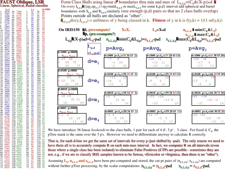
Form Class Hulls using linear d boundaries thru min and max of Lk.d,p=(Ck&(X-p))od On every Ik,p,d{[epi,epi+1) | epj=minLk,p,d or maxLk,p,d for some k,p,d} interval add spherical and barrel boundaries with Sk,p and Rk,p,d similarly (use enough (p,d) pairs so that no 2 class hulls overlap) Points outside all hulls are declared as "other". all p,ddis(y,Ik,p,d) = unfitness of y being classed in k. Fitnessof y in k is f(y,k) = 1/(1-uf(y,k)) On IRIS150 d, precompute! XoX, Ld=Xod nk,L,d min(Ck&Ld) 1 2 3 4 5 6 7 8 9 10 11 12 13 14 15 16 17 18 19 20 21 22 23 24 25 26 27 28 29 30 31 32 33 34 35 36 37 38 39 40 41 42 43 44 45 46 47 48 49 50 51 52 53 54 55 56 57 58 59 60 61 62 63 64 65 66 67 68 69 70 71 72 73 74 75 1 2 3 4 5 6 7 8 9 10 11 12 13 14 15 16 17 18 19 20 21 22 23 24 25 26 27 28 29 30 31 32 33 34 35 36 37 38 39 40 41 42 43 44 45 46 47 48 49 50 51 52 53 54 55 56 57 58 59 60 61 62 63 64 65 66 67 68 69 70 71 72 73 74 75 Ld 51 49 47 46 50 54 46 50 44 49 54 48 48 43 58 57 54 51 57 51 54 51 46 51 48 50 50 52 52 47 48 54 52 55 49 50 55 49 44 51 50 45 44 50 51 48 51 46 53 50 70 64 69 55 65 57 63 49 66 52 50 59 60 61 56 67 56 58 62 56 59 61 63 61 64 XoX 4026 3501 3406 3306 3996 4742 3477 3885 2977 3588 4514 3720 3401 2871 5112 5426 4622 4031 4991 4279 4365 4211 3516 4004 3825 3660 3928 4158 4060 3493 3525 4313 4611 4989 3588 3672 4423 3588 3009 3986 3903 2732 3133 4017 4422 3409 4305 3340 4407 3789 8329 7370 8348 5323 7350 6227 7523 4166 7482 5150 4225 6370 5784 6967 5442 7582 6286 5874 6578 5403 7133 6274 7220 6858 6955 76 77 78 79 80 81 82 83 84 85 86 87 88 89 90 91 92 93 94 95 96 97 98 99 100 101 102 103 104 105 106 107 108 109 110 111 112 113 114 115 116 117 118 119 120 121 122 123 124 125 126 127 128 129 130 131 132 133 134 135 136 137 138 139 140 141 142 143 144 145 146 146 148 149 150 7366 7908 8178 6691 5250 5166 5070 5758 7186 6066 7037 7884 6603 5886 5419 5781 6933 5784 4218 5798 6057 6023 6703 4247 5883 9283 7055 9863 8270 8973 11473 5340 10463 8802 10826 8250 7995 8990 6774 7325 8458 8474 12346 11895 6809 9563 6721 11602 7423 9268 10132 7256 7346 8457 9704 10342 12181 8500 7579 7729 11079 8837 8406 5148 9079 9162 8852 7055 9658 9452 8622 7455 8229 8445 7306 xk,L,d max(Ck&Ld) d=1000 66 68 67 60 57 55 55 58 60 54 60 67 63 56 55 55 61 58 50 56 57 57 62 51 57 63 58 71 63 65 76 49 73 67 72 65 64 68 57 58 64 65 77 77 60 69 56 77 63 67 72 62 61 64 72 74 79 64 63 61 77 63 64 60 69 67 69 58 68 67 67 63 65 62 59 76 77 78 79 80 81 82 83 84 85 86 87 88 89 90 91 92 93 94 95 96 97 98 99 100 101 102 103 104 105 106 107 108 109 110 111 112 113 114 115 116 117 118 119 120 121 122 123 124 125 126 127 128 129 130 131 132 133 134 135 136 137 138 139 140 141 142 143 144 145 146 146 148 149 150 Lp,d =Ld-pod d=e1 d=e2 d=e3 d=e4 d=1000 p=0000 nk,L,d xk,L,d S 43 58 E 49 70 I 49 79 d=1000 p=AS=(50 34 15 2) d=1000 p=AE=(59 28 43 13) d=1000 p=AI=(66 30 55 20) -7 8 -1 20 -1 29 -16 -1 -10 11 -10 20 -23 -8 -17 4 -17 13 d=0100 p=0000 nk,L,d xk,L,d S 23 44 E 20 34 I 22 38 d=0100 p=AS=(50 34 15 2) d=0100 p=AE=(59 28 43 13) d=0100 p=AI=(66 30 55 20) d=0010 p=0000 nk,L,d xk,L,d -5 16 -8 6 -6 10 -7 14 -10 4 -8 8 -11 10 -14 0 -12 4 S 10 19 E 30 51 I 18 69 d=0010 p=AS=(50 34 15 2) d=0010 p=AE=(59 28 43 13) d=0010 p=AI=(66 30 55 20) d=0001 p=0000 nk,L,d xk,L,d -33 -24 -13 8 -25 26 -45 -36 -25 -4 -37 14 -5 4 15 36 3 54 S 1 6 E 10 18 I 14 25 d=0001 p=AS=(50 34 15 2) d=0001 p=AE=(59 28 43 13) d=0001 p=AI=(66 30 55 20) -1 4 8 16 12 23 -12 -7 -3 5 1 12 -25 -20 -16 -8 -12 -1 FAUST Oblique, LSR Linear, Spherical, Radial classifier p,(pre-ccompute?) Ld,p(X-p)od=Ld-pod nk,L,d,pmin(Ck&Ld,p)=nk,L,d-pod xk,L,d.pmax(Ck&Ld,p)=xk,L,d-pod p=AvgS p=AvgE p=AvgI We have introduce 36 linear bookends to the class hulls, 1 pair for each of 4 ds, 3 ps , 3 class. For fixed d, Ck, the pTree mask is the same over the 3 p's. However we need to differentiate anyway to calculate R correctly. That is, for each d-line we get the same set of intervals for every p (just shifted by -pod). The only reason we need to have them all is to accurately compute R on each min-max interval. In fact, we computer R on all intervals (even those where a single class has been isolated) to eliminate False Positives (if FPs are possible - sometimes they are not, e.g., if we are to classify IRIS samples known to be Setosa, vErsicolor or vIriginica, then there is no "other"). Assuming Ld, nk,L,d and xk,L,d have been pre-computed and stored, the cut-pt pairs of (nk,L,d,p; xk,L,d,p) are computed without further pTree processing, by the scalar computations: nk,L,d,p = nk,L,d-pod xk,L,d.p = xk,L,d-pod.
Analyze R:RnR1 (and S:RnR1?) projections on each interval formed by consecutive L:RnR1 cut-pts. LARC IRIS150-R Sp (X-p)o(X-p) = XoX + L-2p + pop nk,S,p = min(Ck&Sp) xk,S,p max(Ck&Sp) Rp,d Sp-L2p,d = L-2p-(2pod)d + pop + pod2 + XoX - L2dnk,R,p,d = min(Ck&Rp,d) xk,R,p,d max(Ck&Rp,d) 34 246 24 126 2 1 132 730 1622 2281 26 32 0 342610 388 1369 34 246 0 279 5 171 186 748 998 26 32 1 517,4 79 633 16 1641 2391 12 17 220 16 723 1258 12 249 794 16 0 128 34 0 99 393 1096 1217 1826 24 6 12 2081 3445 26 32 270 792 26 5 1558 2568 d=1000 p=AS=(50 34 15 2) d=1000 p=AE=(59 28 43 13) d=1000 p=AI=(66 30 55 20) with AI 17 220 with AE 1 517,4 78 633 -7 8 -1 20 -1 29 -16 -1 -10 11 -10 20 -23 -8 -17 4 -17 13 What is the cost for these additional cuts (at new p-values in an L-interval)? It looks like: make the one additional calculation: L-2p-(2pod)d then AND the interval masks, then AND the class masks? (Or if we already have all interval-class mask, only one mask AND step.) eliminates FPs better? Recursion works wonderfully on IRIS: The only hull overlaps after only d=1000 are And the 4 i's common to both are {i24 i27 i28 i34}. We could call those "errors". 7 4 36 540,4 72 170 If on the L 1000,avgE interval, [-1, 11) we recurse using SavgI we get Ld d=1000 p=origin Setosa 43 58 vErsicolor 49 70 vIrginica 49 79 If we have computed, S:RnR1, how can we utilize it?. We can, of course simply put spherical hulls boundaries by centering on the class Avgs, e.g., Sp p=AvgS Setosa 0 154 E=50 I=11 vErsicolor 394 1767 vIrginica 369 4171 Thus, for IRIS at least, with only d=e1=(1000), with only the 3 ps avgS, avgE, avgI, using full linear rounds, 1 R round on each resulting interval and 1 S, the hulls end up completely disjoint. That's pretty good news! There is a lot of interesting and potentially productive (career building) engineering to do here. What is precisely the best way to intermingle p, d, L, R, S? (minimizing time and False Positives)?
MS: while here is a randomly chosen high ranked (and correctly classified) one.. |From: hallg@lead.egr.msu.edu (Gregory Hall) Subject: Re: Wings News and Playoff Thoughts Organization: College of Engineering, Michigan State University Lines: 16 Distribution: world NNTP-Posting-Host: lead.egr.msu.edu |> As far as Cheveldae is concerned, he is a decent goalie. The most logical > trade in the offseason to me would be between Detroit and NY Rangers. I'm sure |> if Beezer would be traded he would enjoy the opportunity to go back to his |> roots in Detroit. He would be a valuable asset to the Wings and Perhaps the |> Rangers could get a Zombo in return? Beezer got a few good years in him and |> the opportunity to get a fresh start would energize his play. |> Only problem is that Zombo was traded to St. Louis last year for goalie Vincent Riendeau. I think that while Chevy is not among the elite class of goalies, he is adequate given the offensive firepower of the Wings. Greg MS: Here’s a randomly chosen low ranked (correctly classified) hockey article: From: archer@elysium.esd.sgi.com (Archer (Bad Cop) Surly) Subject: Re: SHARKS: Kingston Fired!!! Organization: Silicon Graphics, Inc. Mountain View, CA Lines: 20 In <1993Apr22.212219.23130@iscnvx.lmsc.lockheed.com> spiegel@sgi501.msd.lmsc.lockheed.com (Mark Spiegel) writes: *In article <1993Apr21.234022.2880@CSD-NewsHost.Stanford.EDU> nlu@Xenon.Stanford.EDU (Nelson Lu) writes: *> *>McGill/Hammond -> Johan Garpenlov. Would you really rather have those two *>instead of Johan? * * By your logic then you enjoy having Falloon and Ozolinsh on * injured reserve? * Falloon was hurt on a clean check. He just fell poorly. Same with Wilson. I don't know about Ozolinsh. A judo coach would do more for the Sharks injury situation than Bob Probert. Actually, a judo/ju-jitsu coach could help add a really interesting wrinkle to anyone's game.... MS: Seems pretty reasonable to me… again, both were matches but even a casual observer would see the second, high ranked one, is a much more certain match. By the way, here’s a random mis-classified (but very low ranked) post from the above list – should have been in misc.forsale but was put into rec.sports.hockey. Seems like a pretty honest error… From: psr@acsu.buffalo.edu (Strider) Subject: WANTED: roller-blades Organization: UB Lines: 14 Nntp-Posting-Host: autarch.acsu.buffalo.edu I'm looking for a pair of inline skates (aka roller blades) new or used for less than $60.00 including shipping. Size 11. Strider | SUNY @ Buffalo | psr@acsu.buffalo.edu Lord Mayor, The Hill People | (716) 636 4862 | V127MHSK@ubvms.bitnet "Son, I am able," she said, "though you scare me." "Watch," said I, "beloved." -- Strider | SUNY @ Buffalo | psr@acsu.buffalo.edu Lord Mayor, The Hill People | (716) 636 4862 | V127MHSK@ubvms.bitnet "Son, I am able," she said, "though you scare me." "Watch," said I, "beloved." MS : I’ll be starting in earnest on the clustering coding to get it going, the hard parts will be to figure out how to parallel distribute the processing, and how to efficiently code the abrupt change finder… WP: You may already have this in code (or in mind) but, I think the existing UDR (Univariate Distribution Revealer) process can be modified to identify abrupt distribution changes (as the intervals over which we count 1’s get smaller and smaller (i.e., as we AND in more and more bitslices), an abrupt change reveals itself more and more clearly as an abrupt change in the 1-count over adjacent intervals. Ultimately, if we continue all the way down to singleton intervals (units bitslice) then we have full “count change” info. MS: As an FYI also, we were asked to come up with a way of “rating” fitness of oblique. I’m not sure how academically sound this is, but it seems to work somewhat in practice – wanted to get your view on this.... What I did was to capture for each classified result the worst oblique against all other classes (meaning most orthogonal). I took average and deviation of these “worst” matches and then used a CDF to rank them. It turns out that the bad matches seems to end up on the low ranking side, with the high probability ones always correct. For example, here’s a sampling of matches from the 20newsgroup rec.sports.hockey group with the probability added (I highlighted the classification mistakes). You can see the bad matches are down in the 9-10% range, while the correct ones are always [much] higher. There’s probably an interesting subject for someone in this…. Even the low ranked hockey articles you’d be hard-pressed to out of the blue identify them as hockey related. {"/home/sampleData/20news-bydate-test/rec.sport.hockey/54027": 0.15231481}, {"/home/sampleData/20news-bydate-test/rec.sport.hockey/54119": 0.35247093}, {"/home/sampleData/20news-bydate-test/rec.sport.hockey/54544": 0.23036723}, {"/home/sampleData/20news-bydate-test/rec.sport.hockey/54526": 0.32508323}, {"/home/sampleData/20news-bydate-test/rec.sport.hockey/54780": 0.8012897}, {"/home/sampleData/20news-bydate-test/rec.sport.hockey/54507": 0.40787128}, {"/home/sampleData/20news-bydate-test/rec.sport.hockey/54288": 0.46169692}, {"/home/sampleData/20news-bydate-test/rec.sport.hockey/54047": 0.6382074}, {"/home/sampleData/20news-bydate-test/sci.med/59587": 0.105100326}, {"/home/sampleData/20news-bydate-test/comp.windows.x/67973": 0.09948618}, {"/home/sampleData/20news-bydate-test/misc.forsale/76586": 0.09817315}, {"/home/sampleData/20news-bydate-test/rec.sport.hockey/54366": 0.5131513}, {"/home/sampleData/20news-bydate-test/rec.sport.hockey/54511": 0.6178235}, {"/home/sampleData/20news-bydate-test/rec.sport.hockey/54258": 0.6951847}, {"/home/sampleData/20news-bydate-test/rec.sport.hockey/54172": 0.24725951}, MS: I’m probably next going to capture the class against which the worst match was made to see what the option was (eg, was it a close call in above case between misc.forsale and rec.sports.hockey?). If I can understand better what drives the decisions, I may be able to improve the results MS: Finally, next is a question. We’ve been asked to represent global position vertically. I remember you did something with traversing polar representations WP: PTM took HTM partitioning and traverse those triangles (linearly order them) in a way that preserves distance fairly well (a good choice for the ordering of the HTM triangulation. MS: – the idea would be that simple ptree math would correspond to distances between points on a globe. Is there a way to do this? WP: PTM simple (so far) is a hierarchical way to represent triangulations of the globe in a table order that has some good properties. I doubt if pTree math will pump out great circle distances tho.
Classification accuracy evaluations are usually based on a “Hold Out” method; from the given Trainingset of already classified objects, ~1/3 are randomly held out as a Testset and the remaining 2/3 are used to develop the model (e.g., FAUST vectors and cutoffs). Variations on Holdout: Random Sampling: Repeat the holdout method k times and average the results. Cross-validation: Divide the Trainingset into k equal-sized subsets. In k separate steps, hold out the next one of those subsets as Testset. Then each object is “tested” just once so the total number of errors / Trainingset_size is the error_rate (and fitness = 1- error_rate?) Bootstrapping: Testset sampling is done 1 at a time with replacement. If |Trainingset|=N, a common bootstap is to sample with replacement N times. That set is used to build the model and the others (those never selected) are the Testset. Statistically the Model-building set of size.632N so 36.8% Testset. Bagging is aggregating multiple bootstraps. Boosting: If more is known about the objects, quality weights can be assigned (some objects are known to be more firmly classified) then fitness can be weighted accordingly. Hi Mark, That makes good sense and your method appears to work out well. Can we characterize it as follows? Classes are C1..Ck and an unclassified object, u, we want a weight function, w(k,u) which measure how incorrect it is to declare u to be in class k. In the literature, this would be found under “fuzzy classification”. If Mi,…,Mk are the means of the classes (or medians), another weight function might be simply, w(k,u)=dist(u,Mk) / SUM(over h)dist(u,Mh) From: Mark Silverman [mailto:msilverman@treeminer.com] Sent: Wednesday, May 07, 2014 9:58 AMTo: Perrizo, WilliamSubject: RE: couple of updates... For this particular test, we’ve already split the dataset into a training and test set. The overall result is that for the dataset in question (20newsgroups) we have about 80% accuracy. Therefore, 20% are not correct. So what was asked was to come up with a “measure” on the classification, a confidence level if you will. Currently, oblique just says “in a class” or “not in a class”, not “barely in the class”, or “no brainer, it is in the class”. My idea was to use the value of the oblique calculation to come up with a way of measuring just how far or close it may be to a neighboring class, and deriving a confidence score from that. From the results below, it seems to be a pretty good proxy for this, as the ones that were miscategorized came up low on the score, while the ones that were correctly categorized come up high.
APPENDIX x (x-p)o(x-p) - (x-p)od2 (x-p)o(x-p) d (x-p)od = |x-p| cos p Then TopKOutliers uses SPTS, Rp,d, which measures Square Radial Reach of each xX from the d-line thru p. (X-p)o(X-p) - [(X-p)od]2 = XoX, -2Xop, Xod pre-computed, then 2 scalar adds, 1 mult., 2 adds XoX+pop-2Xop - [Xod-pod]2 XoX+pop-2Xop - Xod2 - 2pod Xod + pod2 XoX+pop-2Xop - Xod2 - 2pod Xod + pod2+XoX+pop or XoX+pop-2Xop - 2pod Xod + pod2 - Xod2 + XoX FAUST Oblique Analytics:X(X1..Xn)Rn |X|=N, Classes={C1..CK}, d=(d1..dn) |d|=1, p=(p1..pn)Rn, L, R: Lp,d (X-p)od=Xod - pod = Lorigin,d - pod minLp,d,k= min(Lp,d&Ck) maxLp,d,k= max(Lp,d&Ck) Sp (X-p)o(X-p) = XoX + Xo(-2p) + pop minSp,k= min(Sp&Ck) maxSp,k= max(Sp&Ck) Rp,d Sp - Lp,d2 = XoX + Xo(-2p) + pop - L2o,d -2pod*Xod + pod2 = Lo,-2p-(2pod)d + (pop+pod2) + XoX - L2o,d minRp,d,k=min(Rp,d&Ck) maxRp,d,k= max(Rp,d&Ck) FAUST CountChangeClusterer: If DensThres not reached, cut C at PCCsLp,d&C w next (p,d)pdSet FAUST TopKOutliers: Use D2NN=SqDist(x, X')=rank2Sx for TopKOutlier-slider. FAUST PiecewiseLinearClassifier: y is Ck iff yLHk { z | llp.d,k (z-p)od hlp,d,k} (p,d)pdSet LHk is Linear Hull of Class=k, pdSet is chosen set of (p,d) pairs, e.g., (DiagStartPt, Diag). XoD is a central computation for FAUST. e.g., Xod is the only SPTS needed in FAUST CCClusterer and PLClassifier. xX, D2(X,x)=(X-x)o(X-x)=XoX+xox-2Xox. XoX is pre-computed 1 time, then xox is read from XoX, leaving Xox. RkiPTR(x,ptr-RkiD2(X,x)), RkiSD(x,RkiD2(X,x))) vTree (ordered desc on RkiD2(X,x), i=2..q) are constructed. X a hi-value classification trainset (eg, Enron emails), pre-compute? 1. col statistics(min, avg, max, std,...) ; 2. XoX; Xop, p=class_Avg/Median); 3. Xod, d=interclass_Avg/Median_UnitVector; 4. Xox, d2(X,x), Rkid2(X,x), xX, i=2..; 5. Lp,d and Rp,d for all p's and d's above FAUST LinearAndRadialClassifiery is Ck iff yLRHk {z | llp.d,k (z-p)od hlp,d,k AND lrp.d,k (z-p)o(z-p) - (z-p)od2 hrp,d,k(p,d)pdSet }
o=origin; pRn; dRn, |d|=1; {Ck}k=1..K are the classes; An operation enclosed in a parallelogram, , means it is a pTree op, not a scalar operation (on just numeric operands) Lp,d (X - p) o d = Lo,d - [pod] minLp,d,k = min[Lp,d & Ck] maxLp,d,k = max[Lp,d & Ck[ = [minLo,d,k]- pod = [maxLo,d,k] - pod = min(Xod & Ck)- pod = max(Xod & Ck) - podOR = min(X&Ck) o d- pod = max(X&Ck) o d - pod Sp = (X - p)o(X - p) = -2Xop+So+pop = Lo,-2p + (So+pop) minSp,k=minSp&Ck maxSp,k = maxSp&Ck = min[(X o (-2p) &Ck)]+ (XoX+pop) =max[(X o (-2p) &Ck)] + (XoX+pop) OR= min[(X&Ck)o-2p]+ (XoX+pop) =max[(X&Ck)o-2p] + (XoX+pop) Rp,d Sp, - Lp,d2 minRp,d,k=min[Rp,d&Ck] maxRp,d,k=max[Rp,d&Ck] LARC IRIS150-. Consider all 3 functionals, L, S and R. What's the most efficient way to calculate all 3?\ I suggest that we use each of the functionals with each of the pairs, (p,d) that we select for application (since, to get R we need to compute L and S anyway). So it would make sense to develop an optimal (minimum work and time) procedure to create L, S and R for any (p,d) in the set.
C13 C8,1: D=0110 Ch,1: D=10-10 Ca,1: D=0011 Cg,1: D=1-100 Cf,1: D=1111 Ce,1: D=0111 C5,1: D=1100 C6,1: D=1010 C9,1: D=0101 C7,1: D=1001 C2,3: D=0100 Cb,1: D=1110 C3,3: D=0010 Cc,1: D=1101 C4,1: D=0001 Cd,1: D=1011 C1,1: D=1000 55 169 y isa O if yoD(-,55)(169,) L H y isa O|S if yoD Ce,1 [55,169] 81 182 y isa O if yoD(-,81)(182,) L H y isa O|S if yoD Cc,1 [81,182] 68 117 y isa O if yoD(-,68)(117,) L H y isa O|S if yoD C6,1 [68,117] 3 46 y isa O if yoD(-,3)(46,) L H y isa O|S if yoD Ci,1 [3,46] 10 22 y isa O if yoD(-,10)(22,) L H y isa O|S if yoD Ch,1 [10,22] 84 204 y isa O if yoD(-,84)(204,) L H y isa O|S if yoD Cg,1 [84,204] 39 127 y isa O if yoD(-,39)(127,) L H y isa O|S if yoD Cf,1 [39,127] 71 137 y isa O if yoD(-,71)(137,) L H y isa O|S if yoD Cd,1 [71,137] 10 19 y isa O if yoD(-,10)(19,) L H y isa O|S if yoD C4,1 [10,19] 1 6 y isa O if yoD(-,1)(6,) L H y isa O|S if yoD C5,1 [1,6] 23 44 y isa O if yoD(-,23)(44,) L H y isa O|S if yoD C3,3 [23,44] 54 146 y isa O if yoD(-,54)(146,) L H y isa O|S if yoD C7,1 [54,146] 12 91 y isa O if yoD(-,12)(91,) L H y isa O|S if yoD Cb,1 [12,91] 26 61 y isa O if yoD(-,26)(61,) L H y isa O|S if yoD Ca,1 [26,61] 36 105 y isa O if yoD(-,36)(105,) L H y isa O|S if yoD C9,1 [36,105] 44 100 y isa O if yoD(-,44)(100,) L H y isa O|S if yoD C8,1 [44,100] 43 58 y isa O if yoD(-,43)(58,) L H y isa O|S if yoD C2,3 [43,58] 400 1000 1500 2000 2500 3000 LARC on IRIS150 y isa OTHER if yoDse (-,495)(802,1061)(2725,) Dse 9 -6 27 10 495 802 S 1270 2010 E 1061 2725 I L H y isa OTHER or S if yoDse C1,1 [ 495 , 802] y isa OTHER or I if yoDse C1,2 [1061 ,1270] y isa OTHER or E or I if yoDse C1,3 [1270 ,2010 C1,3: 0 s 49 e 11 i y isa OTHER or I if yoDse C1,4 [2010 ,2725] Dei -3 -2 3 3 -117 -44 E y isa O if yoDei (-,-117)(-3,) -62 -3 I y isa O or E or I if yoDei C2,1 [-62 ,-44] L H y isa O or I if yoDei C2,2 [-44 , -3] C2,1: 2 e 4 i Dei 6 -2 3 1 420 459 E y isa O if yoDei (-,420)(459,480)(501,) 480 501 I y isa O or E if yoDei C3,1 [420 ,459] L H y isa O or I if yoDei C3,2 [480 ,501] Continue this on clusters with OTHER + one class, so the hull fits tightely (reducing false positives), using diagonals? The amount of work yet to be done., even for only 4 attributes, is immense.. For each D, we should fit boundaries for each class, not just one class. For 4 attributes, I count 77 diagonals*3 classes = 231 cases. How many in the Enron email case with 10,000 columns? Too many for sure!! D, not only cut at minCoD, maxCoD but also limit the radial reach for each class (barrel analytics)? Note, limiting the radial reach limits all other directions [other than the D direction] in one step and therefore by the same amount. I.e., it limits all directions assuming perfectly round clusters). Think about Enron, some words (columns) have high count and others have low count. Our radial reach threshold would be based on the highest count and therefore admit many false positives. We can cluster directions (words) by count and limit radial reach differently for different clusters??
Dot Product SPTS computation:XoD = k=1..nXkDk D2,0 D2,1 D1,0 D1,1 D X1*X2 = (21 p1,1 +20 p1,0) (21 p2,1 +20 p2,0) = 22 p1,1 p2,1 +21( p1,1 p2,0+ p2,1 p1,0) + 20 p1,0 p2,0 1 1 3 3 1 1 pXoD,1 pXoD,0 pXoD,3 pXoD,2 X X1 X2 p11 p10 p21 p20 XoD 0 1 1 0 1 0 0 1 1 1 1 1 1 1 0 1 1 1 0 1 0 1 1 0 1 0 0 1 0 0 6 9 9 0 1 1 0 1 1 1 3 2 1 0 1 0 1 1 1 1 0 0 0 0 1 0 1 & & & & 0 1 1 0 1 1 1 1 0 1 1 0 1 0 1 1 0 1 0 1 1 0 1 0 pX1*X2,0 0 1 0 pX1*X2,1 0 1 0 0 1 0 X X1 X2 pX1*X2,2 pX1*X2,3 p11 p10 p21 p20 X1*X2 D2,0 D2,1 D1,0 D1,1 D ( ( = 22 = 22 1 p1,1 1 p1,1 + 1 p2,1 ) + 1 p2,1 ) + 1 p2,0 ) + 1 p2,0 ) + 21 (1 p1,0 + 21 (1 p1,0 + 1 p11 + 1 p11 + 20 (1 p1,0 + 20 (1 p1,0 + 1 p2,0 + 1 p2,0 + 1 p2,1 ) + 1 p2,1 ) 1 3 2 1 3 1 0 1 1 1 1 0 0 1 0 1 1 1 1 9 2 1 1 0 0 0 0 0 1 0 1 0 1 1 0 3 3 1 1 & & 0 1 0 0 0 0 0 0 1 CAR12,3 1 1 0 0 1 0 0 0 1 0 1 0 1 0 1 CAR11,2 0 0 0 1 0 0 CAR10,1 CAR22,3 & pX1*X2,1 pX1*X2,2 pX1*X2,3 pX1*X2,0 & & & CAR21,2 0 1 1 0 0 0 1 0 1 0 0 1 0 0 0 1 0 0 0 1 1 1 0 0 CAR13,4 PXoD,0 PXoD,3 PXoD,2 PXoD,1 0 1 0 0 0 0 1 0 1 0 1 0 1 1 0 PXoD,4 0 1 0 0 0 0 0 1 0 0 0 1 0 1 0 Different data. CAR10,1 pTrees XoD 0 0 1 X 0 0 0 1 0 1 0 0 1 0 1 0 0 0 0 1 1 0 0 1 1 1 1 0 0 1 1 0 1 1 1 0 0 0 1 1 0 1 0 1 1 0 1 1 0 1 1 1 0 0 1 1 1 1 0 1 0 0 1 0 1 0 0 1 1 0 0 0 1 0 0 1 1 3 2 1 3 1 0 1 1 1 1 0 0 1 0 1 1 1 6 18 9 PXoD,0 PXoD,2 PXoD,1 PXoD,3 1 1 0 1 1 0 1 1 1 1 0 1 & & & & & & & & & & & & & & /*Calc PXoD,i after PXoD,i-1 CarrySet=CARi-1,i RawSet=RSi */ INPUT: CARi-1,i, RSi ROUTINE: PXoD,i=RSiCARi-1,i CARi,i+1=RSi&CARi-1,i OUTPUT: PXoD,i, CARi,i+1 1 1 0 0 1 1 0 1 1 1 0 1 1 1 0 0 1 1 0 1 1 0 1 0 1 1 1 0 1 0 We have extended the Galois field, GF(2)={0,1}, XOR=add, AND=mult to pTrees. SPTS multiplication: (Note, pTree multiplication = &)
Example: FAUST Oblique: XoD used in CCC, TKO, PLC and LARC) and (x-X)o(x-X) p1 p1 p1 p,0 p,0 p,0 p3 p3 p3 p2 p2 p2 X X1 X2 p11 p10 p21 p20 XoD XoD XoD = -2Xox+xox+XoX is used in TKO. 0 0 0 0 1 1 1 0 0 1 0 1 1 1 0 1 1 1 3 9 2 2 3 3 3 6 5 0 1 0 0 0 0 0 0 0 1 0 1 1 1 0 0 1 1 1 3 2 1 0 1 0 1 1 1 1 0 0 0 0 1 0 1 n=1 p=2 n=0 p=2 P &p0 P=p0&P P p1 P=P&p1 D2,0 D2,0 D2,0 D2,1 D2,1 D2,1 D1,0 D1,0 D1,0 D1,1 D1,1 D1,1 D=x2 D=x1 D=x3 0 1 1 0 1 1 1 1 1 1 1 1 1 1 1 1 1 1 32 1*21+ 22 1*21+1*20=3 so -2x1oX = -6 0 1 0 1 0 0 2 1 1 1 3 0 0 1 1 1 1 0 n=3 p=2 n=2 p=1 n=1 p=1 n=0 p=1 P &p2 P=p'2&P P p3 P &p1 P &p0 P=P&p'3 P=p1&P P=p0&P RankN-1(XoD)=Rank2(XoD) 0 0 0 1 0 1 1 0 1 1 0 1 1 0 1 1 0 0 0 1 0 1 0 1 1 1 0 1 1 1 1 0 1 1 0 1 1<2 2-1=1 0*23+ 0<1 1-0=1 0*23+0*22 21 0*23+0*22+1*21+ 11 0*23+0*22+1*21+1*20=3 so -2x2oX= -6 RankN-1(XoD)=Rank2(XoD) n=2 p=2 n=1 p=2 n=0 p=1 P=p'1&P P &p1 P=P&p2 P=p0&P P p2 P &p0 0 0 1 1 1 0 0 1 1 0 1 1 1 0 1 1 1 1 0 0 1 0 1 1 0 0 1 22 1*22+ 1<2 2-1=1 1*22+0*21 11 1*22+0*21+1*20=5 so -2x3oX= -10 So in FAUST, we need to construct lots of SPTSs of the type, X dotted with a fixed vector, a costly pTree calculation (Note that XoX is costly too, but it is a 1-time calculation (a pre-calculation?). xox is calculated for each individual x but it's a scalar calculation and just a read-off of a row of XoX, once XoX is calculated.. Thus, we should optimize the living he__ out of the XoD calculation!!! The methods on the previous seem efficient. Is there a better method? Then for TKO we need to computer ranks: RankK: p is what's left of K yet to be counted, initially p=K V is the RankKvalue, initially 0. For i=bitwidth+1 to 0 if Count(P&Pi) p { KVal=KVal+2i; P=P&Pi}; else /* < p */ { p=p-Count(P&Pi);P=P&P'i }; RankN-1(XoD)=Rank2(XoD)
pTree Rank(K) computation: (Rank(N-1) gives 2nd smallest which is very useful in outlier analysis?) p1 p,0 p3 p2 X X1 X2 p11 p10 p21 p20 XoD 1 0 0 1 1 1 2 3 3 0 0 0 0 1 1 1 3 2 1 0 1 0 1 1 1 1 0 0 0 0 1 0 1 D2,0 D2,1 D1,0 D1,1 D 0 1 3 3 0 1 RankKval= 0 1 0 0 0 0 0 23 * + 22 * + 21 * + 20 * = 5P=MapRankKPts= ListRankKPts={2} RankN-1(XoD)=Rank2(XoD) n=3 p=2 n=2 p=2 n=1 p=2 n=0 p=2 P &p2 P p3 P &p1 P &p0 1 0 0 0 1 1 0 1 1 1 0 0 0 1 1 1 1 1 0 1 1 0 1 1 22 1*23+ 0<2 2-0=2 1*23+0*22+ 0<2 2-0=2 1*23+0*22+0*21+ 22 1*23+0*22+0*21+1*20=9 0 1 1 0 1 1 0 1 1 0 1 1 P=P&p3 P=p'2&P P=p'1&P P=p0&P Cross out the 0-positions of P each step. (n=3) c=Count(P&P4,3)= 3 < 6 p=6–3=3; P=P&P’4,3 masks off highest 3 (val 8) {0} X P4,3P4,2P4,1 P4,0 0 1 1 1 0 0 0 0 1 0 1 1 1 1 10 5 6 7 11 9 3 1 0 0 0 1 1 0 1 0 1 1 1 0 1 (n=2) c=Count(P&P4,2)= 3 >= 3 P=P&P4,2 masks off lowest 1 (val 4) {1} (n=1) c=Count(P&P4,1)=2 < 3 p=3-2=1; P=P&P'4,1 masks off highest 2 (val8-2=6 ) {0} {1} (n=0) c=Count(P&P4,0 )=1 >= 1 P=P&P4,0 RankKval=0; p=K; c=0; P=Pure1; /*Note: n=bitwidth-1. The RankK Points are returned as the resulting pTree, P*/ For i=n to 0 {c=Count(P&Pi); If (c>=p) {RankVal=RankVal+2i; P=P&Pi}; else {p=p-c;P=P&P'i }; return RankKval, P; /* Above K=7-1=6 (looking for the Rank6 or 6th highest vaue (which is also the 2nd lowest value) */ {0} {1} {0} {1}
applied to S, a column of numbers in bistlice format (an SpTS), will produce the DistributionTree of S DT(S) depth=h=0 15 p6' 1 1 1 1 1 0 0 0 0 0 0 0 0 0 0 5/64 [0,64) p6' 1 1 1 1 1 0 0 0 0 0 0 0 0 0 0 p6' 1 1 1 1 1 0 0 0 0 0 0 0 0 0 0 p6' 1 1 1 1 1 0 0 0 0 0 0 0 0 0 0 p6' 1 1 1 1 1 0 0 0 0 0 0 0 0 0 0 p5' 1 1 1 0 0 1 0 0 0 0 0 0 0 0 1 p5' 1 1 1 0 0 1 0 0 0 0 0 0 0 0 1 p5' 1 1 1 0 0 1 0 0 0 0 0 0 0 0 1 2/32[64,96) p4' 1 0 0 1 0 0 0 0 0 0 1 0 1 0 0 1[32,48) p5' 1 1 1 0 0 1 0 0 0 0 0 0 0 0 1 3/32[0,32) p4' 1 0 0 1 0 0 0 0 0 0 1 0 1 0 0 2[96,112) p4' 1 0 0 1 0 0 0 0 0 0 1 0 1 0 0 0[64,80) p4' 1 0 0 1 0 0 0 0 0 0 1 0 1 0 0 1/16[0,16) p5' 1 1 1 0 0 1 0 0 0 0 0 0 0 0 1 p4' 1 0 0 1 0 0 0 0 0 0 1 0 1 0 0 p5' 1 1 1 0 0 1 0 0 0 0 0 0 0 0 1 p4' 1 0 0 1 0 0 0 0 0 0 1 0 1 0 0 p5' 1 1 1 0 0 1 0 0 0 0 0 0 0 0 1 p6' 1 1 1 1 1 0 0 0 0 0 0 0 0 0 0 p4' 1 0 0 1 0 0 0 0 0 0 1 0 1 0 0 p6' 1 1 1 1 1 0 0 0 0 0 0 0 0 0 0 p4' 1 0 0 1 0 0 0 0 0 0 1 0 1 0 0 p5' 1 1 1 0 0 1 0 0 0 0 0 0 0 0 1 p6' 1 1 1 1 1 0 0 0 0 0 0 0 0 0 0 p4 0 1 1 0 1 1 1 1 1 1 0 1 0 1 1 6[112,128) p4 0 1 1 0 1 1 1 1 1 1 0 1 0 1 1 1[48,64) p3' 0 0 1 1 1 1 1 1 0 1 0 0 0 0 1 1[16,24) p4 0 1 1 0 1 1 1 1 1 1 0 1 0 1 1 2/16[16,32) p4 0 1 1 0 1 1 1 1 1 1 0 1 0 1 1 2[80,96) p4 0 1 1 0 1 1 1 1 1 1 0 1 0 1 1 p4 0 1 1 0 1 1 1 1 1 1 0 1 0 1 1 p4 0 1 1 0 1 1 1 1 1 1 0 1 0 1 1 p4 0 1 1 0 1 1 1 1 1 1 0 1 0 1 1 p5 0 0 0 1 1 0 1 1 1 1 1 1 1 1 0 p5 0 0 0 1 1 0 1 1 1 1 1 1 1 1 0 2/32[32,64) p5 0 0 0 1 1 0 1 1 1 1 1 1 1 1 0 p5 0 0 0 1 1 0 1 1 1 1 1 1 1 1 0 ¼[96,128) p5 0 0 0 1 1 0 1 1 1 1 1 1 1 1 0 p5 0 0 0 1 1 0 1 1 1 1 1 1 1 1 0 p5 0 0 0 1 1 0 1 1 1 1 1 1 1 1 0 p5 0 0 0 1 1 0 1 1 1 1 1 1 1 1 0 p3' 0 0 1 1 1 1 1 1 0 1 0 0 0 0 1 1[48,56) p3 1 1 0 0 0 0 0 0 1 0 1 1 1 1 0 1[24,32) p3 1 1 0 0 0 0 0 0 1 0 1 1 1 1 0 0[56,64) p3' 0 0 1 1 1 1 1 1 0 1 0 0 0 0 1 0[0,8) p3' 0 0 1 1 1 1 1 1 0 1 0 0 0 0 1 1[32,40) p3 1 1 0 0 0 0 0 0 1 0 1 1 1 1 0 1[8,16) p3 1 1 0 0 0 0 0 0 1 0 1 1 1 1 0 0[40,48) p6 0 0 0 0 0 1 1 1 1 1 1 1 1 1 1 10/64 [64,128) p6 0 0 0 0 0 1 1 1 1 1 1 1 1 1 1 p3' 0 0 1 1 1 1 1 1 0 1 0 0 0 0 1 2[80,88) p3' 0 0 1 1 1 1 1 1 0 1 0 0 0 0 1 3[112,120) p6 0 0 0 0 0 1 1 1 1 1 1 1 1 1 1 p6 0 0 0 0 0 1 1 1 1 1 1 1 1 1 1 p6 0 0 0 0 0 1 1 1 1 1 1 1 1 1 1 p6 0 0 0 0 0 1 1 1 1 1 1 1 1 1 1 p6 0 0 0 0 0 1 1 1 1 1 1 1 1 1 1 p6 0 0 0 0 0 1 1 1 1 1 1 1 1 1 1 p3 1 1 0 0 0 0 0 0 1 0 1 1 1 1 0 0[88,96) p3 1 1 0 0 0 0 0 0 1 0 1 1 1 1 0 3[120,128) p3' 0 0 1 1 1 1 1 1 0 1 0 0 0 0 1 p3' 0 0 1 1 1 1 1 1 0 1 0 0 0 0 1 0[96,104) p3 1 1 0 0 0 0 0 0 1 0 1 1 1 1 0 p3 1 1 0 0 0 0 0 0 1 0 1 1 1 1 0 2[194,112) UDR Univariate Distribution Revealer (on Spaeth:) 5 10 depth=h=1 node2,3 [96.128) yofM 11 27 23 34 53 80 118 114 125 114 110 121 109 125 83 p6 0 0 0 0 0 1 1 1 1 1 1 1 1 1 1 p5 0 0 0 1 1 0 1 1 1 1 1 1 1 1 0 p4 0 1 1 0 1 1 1 1 1 1 0 1 0 1 1 p3 1 1 0 0 0 0 0 0 1 0 1 1 1 1 0 p2 0 0 1 0 1 0 1 0 1 0 1 0 1 1 0 p1 1 1 1 1 0 0 1 1 0 1 1 0 0 0 1 p0 1 1 1 0 1 0 0 0 1 0 0 1 1 1 1 p6' 1 1 1 1 1 0 0 0 0 0 0 0 0 0 0 p5' 1 1 1 0 0 1 0 0 0 0 0 0 0 0 1 p4' 1 0 0 1 0 0 0 0 0 0 1 0 1 0 0 p3' 0 0 1 1 1 1 1 1 0 1 0 0 0 0 1 p2' 1 1 0 1 0 1 0 1 0 1 0 1 0 0 1 p1' 0 0 0 0 1 1 0 0 1 0 0 1 1 1 0 p0' 0 0 0 1 0 1 1 1 0 1 1 0 0 0 0 Y y1 y2 y1 1 1 y2 3 1 y3 2 2 y4 3 3 y5 6 2 y6 9 3 y7 15 1 y8 14 2 y9 15 3 ya 13 4 pb 10 9 yc 11 10 yd 9 11 ye 11 11 yf 7 8 3 2 2 8 f= 1 2 1 1 0 2 2 6 0 1 1 1 1 0 1 000 2 0 0 2 3 3 depthDT(S)b≡BitWidth(S) h=depth of a node k=node offset Nodeh,k has a ptr to pTree{xS | F(x)[k2b-h+1, (k+1)2b-h+1)} and its 1count Pre-compute and enter into the ToC, all DT(Yk) plus those for selected Linear Functionals (e.g., d=main diagonals, ModeVector . Suggestion: In our pTree-base, every pTree (basic, mask,...) should be referenced in ToC( pTree, pTreeLocationPointer, pTreeOneCount ).and these OneCts should be repeated everywhere (e.g., in every DT). The reason is that these OneCts help us in selecting the pertinent pTrees to access - and in fact are often all we need to know about the pTree to get the answers we are after.).
D2,0 D2,1 D1,0 D1,1 D So let us look at ways of doing the work to calculate As we recall from the below, the task is to ADD bitslices giving a result bitslice and a set of carry bitslices to carry forward XoD = k=1..nXk*Dk 1 1 3 3 1 1 ( ( = 22 = 22 1 p1,1 1 p1,1 + 1 p2,1 ) + 1 p2,1 ) ( ( ( ( + 1 p2,0 ) + 1 p2,0 ) 1 p1,0 1 p1,0 + 1 p11 + 1 p11 1 p1,0 1 p1,0 + 21 + 21 + 1 p2,0 + 1 p2,0 + 1 p2,1 ) + 1 p2,1 ) + 20 + 20 pTrees XoD X 1 0 0 1 0 0 0 1 1 0 1 1 1 3 2 1 0 1 0 1 1 1 1 0 0 0 0 1 0 1 6 9 9 0 1 1 0 1 1 1 1 0 1 1 0 1 0 1 1 0 1 0 1 1 1 1 1 1 0 0 I believe we add by successive XORs and the carry set is the raw set with one 1-bit turned off iff the sum at that bit is a 1-bit Or we can characterize the carry as the raw set minus the result (always carry forward a set of pTrees plus one negative one). We want a routine that constructs the result pTree from a positive set of pTrees plus a negative set always consisting of 1 pTree. The routine is: successive XORs across the positive set then XOR with the negative set pTree (because the successive pset XOR gives us the odd values and if you subtract one pTree, the 1-bits of it change odd to even and vice versa.): /*For PXoD,i (after PXoD,i-1). CarrySetPos=CSPi-1,i CarrySetNeg=CSNi-1,i RawSet=RSi CSP-1=CSN-1=*/ INPUT: CSPi-1, CSNi-1, RSi ROUTINE: PXoD,i=RSiCSPi-1,iCSNi-1,i CSNi,i+1=CSNi-1,iPXoD,i; CSPi,i+1=CSPi-1,iRSi-1; OUTPUT: PXoD,i, CSNi,i+1 CSPi,i+1 0 1 1 0 1 1 1 1 0 0 0 0 1 0 1 1 1 0 1 0 1 CSN-1.0PXoD,0 CSP-1,0RS0 RS1 CSN0,1= CSP0,1= CSP-1,0=CSN-1,0= RS0 PXoD,0 PXoD,1 1 1 0 1 0 1 0 1 1 1 1 0 0 1 1 0 1 1 1 0 1 0 0 0 1 1 0 1 0 1 = = 1 0 1 0 0 0 0 1 1 1 0 1 0 0 0
D2,0 D2,0 D2,1 D2,1 D1,0 D1,0 D1,1 D1,1 D D XoD = k=1..nXk*Dk 1 1 1 0 3 3 1 2 1 1 0 1 k=1..n ( = 22B Dk,B pk,B k=1..n ( Dk,B pk,B-1 + Dk,B-1 pk,B + 22B-1 k=1..n ( Dk,B pk,B-2 + Dk,B-1 pk,B-1 + Dk,B-2 pk,B + 22B-2 Xk*Dk = Dkb2bpk,b XoD=k=1,2Xk*Dk with pTrees: qN..q0, N=22B+roof(log2n)+2B+1 k=1..n ( +Dk,B-3 pk,B Dk,B pk,B-3 + Dk,B-1 pk,B-2 + Dk,B-2 pk,B-1 + 22B-3 = Dk(2Bpk,B +..+20pk,0) = (2BDk,B+..+20Dk,0) (2Bpk,B +..+20pk,0) . . . k=1..2 ( = 2BDkpk,B +..+ 20Dkpk,0 = 22 Dk,1 pk,1 k=1..n ( Dk,Bpk,B) = 22B( +Dk,Bpk,B-1) + 22B-1(Dk,B-1pk,B Dk,B pk,0 + Dk,2 pk,1 + Dk,1 pk,2 +Dk,0 pk,3 + 23 +..+20Dk,0pk,0 k=1..2 ( Dk,1 pk,0 + Dk,0 pk,1 + 21 pTrees k=1..n ( X Dk,2 pk,0 + Dk,1 pk,1 + Dk,0 pk,2 + 22 B=1 1 3 2 1 0 1 0 1 1 1 1 0 0 0 0 1 0 1 k=1..2 ( k=1..n ( Dk,0 pk,0 Dk,1 pk,0 + Dk,0 pk,1 + 20 + 21 q0 = p1,0 = no carry 1 1 0 k=1..n ( Dk,0 pk,0 + 20 ( ( = 22 = 22 1 p1,1 D1,1p1,1 + 1 p2,1 ) + D2,1p2,1 ) ( ( ( ( + 1 p2,0 ) + D2,0p2,0) D1,1p1,0 1 p1,0 + 1 p11 + D1,0p11 1 p1,0 D1,0p1,0 + 21 + 21 + 1 p2,0 + D2,1p2,0 + 1 p2,1 ) + D2,0p2,1) + 20 + 20 q1= carry1= 1 1 0 0 0 1 ( = 22 D1,1 p1,1 + D2,1 p2,1 ) ( ( + D2,0 p2,0) D1,1 p1,0 +D1,0 p11 D1,0 p1,0 + 21 + D2,1 p2,0 +D2,0 p2,1) + 20 0 0 0 q2=carry1= no carry 0 1 1 1 0 1 1 1 0 0 0 1 q0 = carry0= 0 1 1 1 0 0 0 1 1 0 1 1 1 1 0 0 0 0 1 1 0 1 0 1 1 0 1 1 1 1 2 1 1 q1=carry0+raw1= carry1= 1 1 1 1 1 1 q2=carry1+raw2= carry2= 1 1 1 q3=carry2 = carry3= A carryTree is a valueTree or vTree, as is the rawTree at each level (rawTree = valueTree before carry is incl.). In what form is it best to carry the carryTree over? (for speediest of processing?) 1. multiple pTrees added at next level? (since the pTrees at the next level are in that form and need to be added) 2. carryTree as a SPTS, s1? (next level rawTree=SPTS, s2, then s10& s20 = qnext_level and carrynext_level ? CCC ClustererIf DT (and/or DUT) not exceeded at C, partition C further by cutting at each gap and PCC in CoD For a table X(X1...Xn), the SPTS, Xk*Dk is the column of numbers, xk*Dk. XoD is the sum of those SPTSs, k=1..nXk*Dk So, DotProduct involves just multi-operand pTree addition. (no SPTSs and no multiplications) Engineering shortcut tricka would be huge!!!
Question: Which primitives are needed and how do we compute them? X(X1...Xn) D2NN yields a 1.a-type outlier detector (top k objects, x, dissimilarity from X-{x}). D2NN = each min[D2NN(x)] (x-X)o(x-X)= k=1..n(xk-Xk)(xk-Xk)=k=1..n(b=B..02bxk,b-2bpk,b)( (b=B..02bxk,b-2bpk,b) ----ak,b--- b=B..02b(xk,b-pk,b) ) ( 22Bak,Bak,B + =k=1..n( b=B..02b(xk,b-pk,b) )( 22B-1( ak,Bak,B-1 + ak,B-1ak,B ) + { 22Bak,Bak,B-1 } =k (2Bak,B+ 2B-1ak,B-1+..+ 21ak, 1+ 20ak, 0) (2Bak,B+ 2B-1ak,B-1+..+ 21ak, 1+ 20ak, 0) 22B-2( ak,Bak,B-2 + ak,B-1ak,B-1 + ak,B-2ak,B ) + {2B-1ak,Bak,B-2 + 22B-2ak,B-12 22B-3( ak,Bak,B-3 + ak,B-1ak,B-2 + ak,B-2ak,B-1 + ak,B-3ak,B ) + { 22B-2( ak,Bak,B-3 + ak,B-1ak,B-2 ) } 22B-4(ak,Bak,B-4+ak,B-1ak,B-3+ak,B-2ak,B-2+ak,B-3ak,B-1+ak,B-4ak,B)... {22B-3( ak,Bak,B-4+ak,B-1ak,B-3)+22B-4ak,B-22} =22B ( ak,B2 + ak,Bak,B-1 ) + 22B-1( ak,Bak,B-2 ) + 22B-2( ak,B-12 + ak,Bak,B-3 + ak,B-1ak,B-2 ) + 22B-3( ak,Bak,B-4+ak,B-1ak,B-3) + 22B-4ak,B-22 ... X(X1...Xn) RKN (Rank K Nbr), K=|X|-1, yields1.a_outlier_detector (top y dissimilarity from X-{x}). ANOTHER TRY! Install in RKN, each RankK(D2NN(x)) (1-time construct but for. e.g., 1 trillion xs? |X|=N=1T, slow. Parallelization?) xX, the square distance from x to its neighbors (near and far) is the column of number (vTree or SPTS) d2(x,X)= (x-X)o(x-X)= k=1..n|xk-Xk|2= k=1..n(xk-Xk)(xk-Xk)= k=1..n(xk2-2xkXk+Xk2) Should we pre-compute all pk,i*pk,j p'k,i*p'k,j pk,i*p'k,j D2NN=multi-op pTree adds? When xk,b=1, ak,b=p'k,b and when xk,b=0, ak,b= -pk.b So D2NN just multi-op pTree mults/adds/subtrs? Each D2NN row (each xX) is separate calc. = -2 kxkXk + kxk2 + kXk2 3. Pick this from XoX for each x and add to 2. = -2xoX + xox + XoX 5. Add 3 to this k=1..n i=B..0,j=B..02i+jpk,ipk,j 1. precompute pTree products within each k i,j 2i+j kpk,ipk,j 2. Calculate this sum one time (independent of the x) -2xoX cost is linear in |X|=N. xox cost is ~zero. XoX is 1-time -amortized over xX (i.e., =1/N) or precomputed The addition cost, -2xoX + xox + XoX, is linear in |X|=N So, overall, the cost is linear in |X|=n. Data parallelization? No! (Need all of X at each site.) Code parallelization? Yes! (After replicating X to all sites, Each site creates/saves D2NN for its partition of X, then sends requested number(s) (e.g., RKN(x) ) back.
LARC on IRIS150-3 Here we use the diagonals. d=e1 p=AVGs, L=(X-p)od 43 58 S 49 70 E 49 79I R(p,d,X) SEI 0 128 270 393 1558 3444 [43,49) S(16) 0 128 [49,58) E(24)I(6) 0 S(34) 99 393 1096 1217 1825 [70,79] I(12) 2081 3444 [58,70) E(26) I(32) 270 792 1558 2567 E(50) I(7) 49 49 (36,7) 63 70 (11) Only overlap L=[58,70), R[792,1557] (E(26),I(5)) With just d=e1, we get good hulls using LARC: While Ip,d containing >1class, for next (d,p) create L(p,d)Xod-pod, R(p,d)XoX+pop-2Xop-L2 1. MnCls(L), MxCls(L), create a linear boundary. 2. MnCls(R), MxCls(R).create a radial boundary. 3. Use R&Ck to create intra-Ck radial boundaries Hk = {I | Lp,d includes Ck} R & L I(1) I(42)
y isa O if yoD (-,-2) (19,) y isa O or I(8) if yoD [ -2 , 1.4] y isa O or E(40) or I(2) if yoD C3,1 [ 1.4 ,19] y isa O if y isa C3,1 AND SRR(AVGs,Dei)[0,2)(370,) y isa O or E(4) if y isa C3,1 AND SRR(AVGs,Dei)[2,8) y isa O or E(27) or I(2) if y isa C3,1 AND SRR(AVGs,Dei)[8,106) y isa O or E(9) if y isa C3,1 AND SRR(AVGs,Dei)[106,370] LARC on IRIS150 y isa O if yoD (-,-184)(123,381)(2046,) y isa O or S(50) if yoD C1,1 [-184 , 123] Dse 9 -6 27 10; xoDes: -184 123 S 590 1331 E 381 2046 I y isa O or I(1) if yoD C1,2 [ 381 , 590] y isa O or E(50) or I(11) if yoD C1,3 [ 590 ,1331] y isa O or I(38) if yoD C1,4 [1331 ,2046] y isa O if y isa C1,1 AND SRR(AVGs,Dse)(154,) y isa O or S(50) if y isa C1,1 AND SRR(AVGs,DSE)[0,154] SRR(AVGs,dse) on C1,1 0 154 S SRR(AVGs,dse) on C1,2 only one such I y isa O if y isa C1,3 AND SRR(AVGs,Dse)(-,2)U(143,) y isa O or E(10) if y isa C1,3 AND SRR in [2,7) y isa O or E(40) or I(10) if y isa C1,3 AND SRR in [7,137) = C2,1 y isa O or I(1) if y isa C1,3 AND SRR in [137,143] etc. SRR(AVGs,dse) onC1,3 2 137 E 7 143 I Dei 1 .7 -7 -4; xoDei on C2,1: 1.4 19 E -2 3 I SRR(AVGe,dei) onC3,1 2 370 E 8 106 I We use the Radial steps to remove false positives from gaps and ends. We are effectively projecting onto a 2-dim range, generated by the Dline and the Dline (which measures the perpendicular radial reach from the D-line). In the D projections, we can attempt to cluster directions into "similar" clusters in some way and limit the domain of our projections to one of these clusters at a time, accommodating "oval" shaped or elongated clusters giving a better hull fit. E.g., in the Enron email case the dimensions would be words that have about the same count, reducing false positives.
LARC on IRIS150-2 We use the diagonals. Also we set a MinGapThreshold=2 which will mean we stay 2 units away from any cut y isa O if yoD(-,43)(79,) y isa O or S( 9) if yoD[43,47] y isa O if yoD[43,47]&SRR(-,52)(60,) y isa O or S(41) or E(26) or I( 7) if yoD(47,60) (yC1,2) d=e1=1000; The xod limits: 43 58 S 49 70 E 49 79 I y isa O or E(24) or I(32) if yoD[60,72] (yC1,3) y isa O or I(11) if yoD(72,79] y isa O if yoD[72,79]&SRR(-,49)(78,) y isa O if yoD(-,18)(46,) y isa O or E( 3) if yoD[18,23) y isa O if yoD[18,23)&SRR[0,21) y isa O or E(13) or I( 4) if yoD[23,28) (yC2,1) d=e2=0100 on C1,2 xod lims: 30 44 S 20 32 E 25 30 I y isa O or S(13) or E(10) or I( 3) if yoD[28,34) (yC2,2) y isa O or S(28) if yoD[34,46] y isa O if yoD[34,46]&SRR[0,32][46,) y isa O or E(17) if yoD[60,72]&SRR[1.2,20] d=e2=0100 on C1,3 xod lims: 22 34 E 22 34 I zero differentiation! y isa O or E( 7) or I( 7)if yoD[60,72]&SRR[20, 66] y isa O or I(25)if yoD[60,72]&SRR[66,799] y isa O if yoD[0,1.2)(799,) d=e3=0010 on C2,2 xod lims: 30 33 S 28 32 E 28 30 I y isa O if yoD(-,28)(33,) y isa O or S(13) or E(10) or I(3) if yoD[28,33] y isa O if yoD(-,1)(5,12)(24,) y isa O or S(13) if yoD[1,5] d=e3=0001 xod lims: 12 18 E 18 24 I y isa O or E( 9) if yoD[12,16) y isa O if yoD[12,16)&SRR[0,208)(558,) y isa O or E( 1) or I( 3) if yoD[16,24) y isa O if yoD[16,24)&SRR[0,1198)(1199,1254)1424,) y isa O or E(1) if yoD[16,24)&SRR[1198,1199] y isa O or I(3) if yoD[16,24)&SRR[1254,1424]
LARC IRIS150. d=AvgEAvgI p=AvgE, L=(X-p)od -36 -25 S -14 11 E -17 33I d=AvgSAvgE p=AvgS, L=(X-p)od -6 4 S 18 42 E 11 64I d=AvgSAvgI p=AvgS, L=(X-p)od -6 5 S 17.5 42 E 12 65I [-14,11) (50, 13) 0 2.8 76 134 [11,33] I(36) [-17,-14)] I(1) [17.5,42) (50,12) 4.7 6 192 205 [18,42) (50,11) 2 6.92 133 137 [11,33] I(37) [42,64] 38 [12,17.5)] I(1) [11,18)] I(1) R(p,d,X) S E I 0 2 6 137 154 393 R(p,d,X) S E I .3 .9 4.7 150 204 213 R(p,d,X) S E I 0 2 32 76 357 514 38ambigs 16errs 30ambigs, 5 errs d=e3 p=AvgS, L=(X-p)od -5 5 S&L 15 37 E&L 4 55I&L d=e2 p=AvgS, L=(X-p)od -11 10 S&L -14 0 E&L -13 4I&L d=e4 p=AvgE, L=(X-p)od -13 -7 S&L -3 5 E&L 1 12I&L d=e4 p=AvgS, L=(X-p)od -2 4 S&L 7 16 E&L 11 23I&L d=e1 p=AS L=(X-p)od (-pod=-50.06) -7.06 7.94 S&L -1;06 19.94 E&L -1.06 28.94 I&L -5,4) 47 [4,15) 3 1 [15,37) 50, 15 157 297 536 792 [37,55] I=34 ,-13) 1 -13,-11 0, 2, 1 all=-11 -11,0 29,47,46 0 66 310 352 1749 4104 [0,4) [4, 15 3 6 -2,4) 50 -7] 50 [-3,1) 21 [7,11) 28 [1,5) 22, 16 .7 .7 4.8 4.8 [11,16) 22, 16 11 16 11 16 [16,23] I=34 [5,12] 34 -8,-2 16 [-2,8) 34, 24, 6 0 99 393 1096 1217 1825 [8,20) 26, 32 270 792 1558 2567 [20,29] 12 3, 1 E=32 I=14 E=22 I=16 E=22 I=16 E=32 I=14 E=18 I=12 E=26 I=5 9, 3 1, 1 2, 1 46,11 d=e3 p=AvgE, L=(X-p)od -32 -24 S&L -12 9 E&L -25 27I&L d=e1 p=AE L=(X-p)od (-pod=-59.36) -17 -1 S&L -11 11 E&L -11 20I&L d=e2 p=AvgE, L=(X-p)od -5 `17 S&L -8 7 E&L -6 11I&L ,-25) 48 -25,-12 2 11 -17-11 16 [-11,-1) 33, 21, 3 0 27 107 172 748 1150 [-12,9) 49, 15 2(17) 16 158 199 [9,27] I=34 [-1,11) 26, 32 1 51 79 633 [11,20] I12 ,-6) 1 [-6, -5) 0, 2, 1 15 18 58 59 [-5,7) 29,47, 46 3 58 234 793 1103 1417 [7,11) [11, 15 3 6 1 err E=5 I=3 E=47 I=22 E=22 I=16 E=46 I=14 E=7 I=4 E=39 I=11 E=47 I=12 21, 3 13, 21 E=26 I=11 E=45 I=12 d=e4 p=AvgI, L=(X-p)od -19 -14 S&L -10 -3 E&L -6 5I&L d=e3 p=AvgI, L=(X-p)od -44 -36 S&L -25 -4 E&L -37 14I&L d=e2 p=AvgI, L=(X-p)od -7 `15 S&L -10 4 E&L -8 9I&L d=e1 p=AI L=(X-p)od (-pod=-65.88) -22 -8 S&L -17 4 E&L -17 14I&L ,-25) 48 -25,-12 2 1 1 [-17,-8) 33, 21, 3 38 126 132 730 1622 2181 [-6,-3) 22, 16 same range [5,12] 34 [-25,-4) 50, 15 5 11 318 453 [9,27] I=34 [-8,4) 26, 32 0 34 1368 730 [-8, -7) 2, 1 allsame [5, 9] 9, 2, 1 allsame ,-6) 1 [-7, 4) 29,46,46 5 36 929 1403 1893 2823 [6,11) [11, 15 3 6 S=9 E=2 I=1 E=2 I=1 E=2 I=1 d=e1 p=AvgS, L=Xod 43 58 S&L 49 70 E&L 49 79 I&L Note that each L=(X-p)od is just a shift of Xod by -pod (for a given d). Next, we examine: For a fixed d, the SPTS, Lp,d. is just a shift of LdLorigin,d by -pod we get the same intervals to apply R to, independent of p (shifted by -pod). Thus, we calculate once, lld=minXod hld=maxXod, then for each different p we shift these interval limit numbers by -pod since these numbers are really all we need for our hulls (Rather than going thru the SPTS calculation of (X-p)od anew new p). There is no reason we have to use the same p on each of those intervals either. So on the next slide, we consider all 3 functionals, L, S and R. E.g., Why not apply S first to limit the spherical reach (eliminate FPs). S is calc'ed anyway?
LARC IRIS150-2 Here we try using other p points for the R step (other than the one used for the L step). d=e4 p=AvgS, L=(X-p)od -2 4 S&L 7 16 E&L 11 23I&L d=e4 p=AvgS, L=(X-p)od -2 4 S&L 7 16 E&L 11 23I&L 30ambigs, 5 errs -2,4) 50 -2,4) 50 [7,11) 28 [7,11) 28 [11,16) 22, 16 5.7 36.2 151.06 611 [11,16) 22, 16 127.5 648.7 1554.7 2892 [16,23] I=34 [16,23] I=34 d=e1 p=AS L=(X-p)od (-pod=-50.06) -7.06 7.94 S&L -1;06 19.94 E&L -1.06 28.94 I&L d=e1 p=AS L=(X-p)od (-pod=-50.06) -7.06 7.94 S&L -1;06 19.94 E&L -1.06 28.94 I&L d=e1 p=AS L=(X-p)od (-pod=-50.06) -7.06 7.94 S&L -1;06 19.94 E&L -1.06 28.94 I&L -8,-2 16 [-2,8) 34, 24, 6 0 99 393 1096 1217 1825 [8,20) 26, 32 270 792 1558 2567 [20,29] 12 E=22 I=7 p=AvgS E=17 I=7 p=AvgE E=22 I=8 p=AvgI E=26 I=5 p=AvgS -8,-2 16 -8,-2 16 [-2,8) 34, 24, 6 0 99 393 1096 1217 1825 [-2,8) 34, 24, 6 0 99 393 1096 1217 1825 [8,20) w p=AvgI 26, 32 0.62 34.9 387.8 1369 [8,20) w p=AvgE 26, 32 1.9 51.8 78.6 633 [20,29] 12 [20,29] 12 <--E=25 I=10 p=AvgI <--E=6 I=4 p=AvgE d=e4 p=AvgS, L=(X-p)od -2 4 S&L 7 16 E&L 11 23I&L [16,23] I=34 -2,4) 50 [7,11) 28 [11,16) 22, 16 127.5 1555 2892 d=e1 p=AvgS, L=Xod 43 58 S&L 49 70 E&L 49 79 I&L There is a best choice of p for the R step (p=AvgE) but how would we decide that ahead of time? For e4, the best choice of p for the R step is also p=AvgE. (There are mistakes in this column on the previous slide!)