Download
1 / 39
390 likes | 653 Views
Exploitation. High. Parasitoids. Parasite. Intimacy. Low. Predator. Grazer. High. Lethality. Low. There are 4 general categories. “True” predators Herbivores Grazers Browsers Granivores Frugivores Parasites Parasitoids. “True” predators. Herbivores. Grazer Browser Granivore

E N D
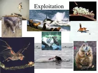
High Parasitoids Parasite Intimacy Low Predator Grazer High Lethality Low
There are 4 general categories • “True” predators • Herbivores • Grazers • Browsers • Granivores • Frugivores • Parasites • Parasitoids
Herbivores • Grazer • Browser • Granivore • Frugivore • Attack many prey items in a lifetime • Consume only a bit of the victim • Do not usually kill prey in the short term (but may do so in the long term)
Parasites • Consume part of their prey • Do not usually kill their prey • Attack one or very few prey items in their lifetime • Parasitoids
Parasites • Parasitoids • which straddle the parasite and true predator categories - they lay eggs inside their host which they eventually kill
Predation is important because: • It may restrict the distribution of, or reduce the abundance of the prey species. • Predation, along with competition, is a major type of interaction that can influence the organization of communities. • Predation is a major selective force, and many adaptations of organisms have their explanation in predator-prey coevolution. • Evolutionary arms race • Predation drives the movement of energy and nutrients in ecosystems.
Vito Volterra(1860-1940) Alfred Lotka(1880-1949)
start Predation • Rate of increase of prey population dH/dt = rH
Predation • Rate of increase of prey population • dH/dt = rH • Predators eat prey • dH/dt = rH-a'HP • a' = capture coefficient • H = Prey pop size • P = Predator pop size
Predation • Rate of increase of predator populations dP/dt = -qP • If only predators exist, no prey, so predators die
Predation • Rate of increase of predator populations dP/dt = -qP • If only predators exist, no prey, so predators die • dP/dt = fa’HP-qP • f = is a predation constant • Predator’s efficiency at turning food into predator offspring. • a' = capture coefficient • q = mortality rate
Predation • Equilibrium population sizes • Predator • dP/dt = fa’HP -qP • 0= fa’HP -qP • fa’HP = qP • fa’H= q • H= q/fa’ • Prey • dH/dt = rH-a’HP • 0= rH-a’HP • rH= a’HP • r = a’P • P = r/ a’
Predation • Graphical Equilibrium • Prey (H) equilibrium (dH/dt=0) is determined by predator population size. • If the predator population size is large the prey population will go extinct • If the predator population is small the prey population size increases Predator Pop size dH/dt =0 r/a’ Prey pop size
Predation dP/dt =0 • Graphical Equilibrium • Predator (P) equilibrium (dP/dt=0) is determined by prey population size. • If the prey population size is large the predator population will increase • If the prey population is small the predator population goes extinct Predator Pop size q/fa’ Prey pop size
Predation dP/dt =0 • Predator-Prey interaction • The stable dynamic of predators and prey is a cycle Predator Pop size r/a’ q/fa’ Prey pop size
Do these models apply to natural populations? • Lynx/Snowshoe Hare - Arctic system where there is one predator and one prey
Lynx/Snowshoe Hare - Arctic system where there is one predator and one preyAssumptions?
Rosenzweig & MacArthur (1963) • Three possible outcomes of interactions • The oscillations are stable (classical oscillations of Lotka-Volterra equations). • The oscillations are damped (convergent oscillation). • The oscillations are divergent and can lead to extinction.
i) Prey iscoline N 2 Predator density Prey increase N K Prey density ii) Predator iscoline 1 1 N 2 K 2 Predator increases Predator decreases Predator density N Prey density 1
a) Damped oscillations Predator isocline Population density Predator Density Prey isocline Prey Density Time Predator-Prey Models • Superimpose prey and predator isoclines • One stable point emerges: the intersection of the lines • Three general cases • Inefficient predators require high densities of prey
Stable oscillations b) Predator equilibrium density Population density Predator Density Prey Density Time Predator-Prey Models • Three general cases (cont.) • A moderately efficient predator leads to stable oscillations of predator and prey populations
Population density Increasing oscillations Predator density Prey Density Time Predator-Prey Models • Three general cases (cont.) • A highly efficient predator can exploit a prey nearly down to its limiting rareness
All these models make a series of simplifying assumptions • A homogenous world in which there are no refuges for the prey or different habitats. • There is one predator species eating one prey species and there are no other species involved in the dynamics of these two populations • Relaxing these assumptions leads to more complex, but more realistic models. • All predators respond to prey in the same fashion regardless of density • Functional Response
Conclusions form field studies • There is not a clear relationship between predator abundance and prey population size. • In some, but not all cases, the abundance of predators does influence the abundance of their prey in field populations.
What makes predators effective in controlling their prey? • Foraging efficieny • Within a patch, the searching efficiency of a predator becomes crucial to its success. • But searching efficiency varies with abiotic factors and can also decrease at high predator densities because of interference of other predators.
Predation • Response of predator to prey density • Numerical • Aggregative • Functional
Types of functional responses • Limited by handling time • The rate of capture by predator • Alters Behavior • Type I • Type II • Type III Eat all you want Eat all you can Eat all you can, if you can find it! C. S. Holling(1930–)
Types of functional responses Slide 25
Keystone predator Bob Paine at University of Washington mussel is a competitive dominant in this system
The effects of herbivory • Individual plants are affected in the following areas • plant defenses • plant compensation • plant growth • plant fecundity
Quantitative Defenses: Prevent digestion as they accumulate in the gut. Usually found in large quantities in the plant parts that are eaten. Most of these compounds are “Carbon Rich” Common defense of plants growing in nutrient poor soils (conifers). Qualitative Defenses: Usually toxic in small quantities. Found in relatively small amounts in the portion of plants that is eaten (leaves). These compounds are “Nitrogen Rich” and therefor expensive to produce by the plant. More common in plants growing on nutrient rich soils. Chemicals Defenses