Download
1 / 10
100 likes | 122 Views
Learn about lossless and dependency-preserving decomposition into 3NF for relational database design. This includes definitions, algorithms, and examples for computing a minimum cover and the 3NF decomposition process.

E N D
10.3 Lossless and dependency-preservingdecomposition into 3NF A lossless and dependency-preserving decomposition into 3NF is always possible. More definitions regarding FD’s are needed. A set F of FD’s is minimal if 1. Every FD X→ Y in F is simple: Y consists of a single attribute, 2. Every FD X→ A in F is left-reduced: there is no proper subset Y⊂X such that X → A can be replaced with Y→A. that is, there is no Y⊂X such that ((F − {X → A}) ∪{Y → A})+ = F+ 3. No FD in F can be removed; that is, there is no FD X→A in F such that (F − {X → A})+ = F+. Iff F |= Y A Iff XA is inferred From F– { XA}
10.3.1 Computing a minimum cover F is a set of FD’s. Aminimal cover (or canonical cover) for F is a minimal set of FD’s Fminsuch that F+= F+min. Algorithm Min_Cover Input: a set F of functional dependencies. Output: a minimum cover of F. Step 1: Reduce right side. Apply Algorithm Reduce right to F. Step 2: Reduce left side. Apply Algorithm Reduce left to the output of Step 2. Step 3: Remove redundant FDs. Apply Algorithm Remove_redundencyto the output of Step 2. The output is a minimum cover. Below we detail the three Steps.
10.3.1 Computing a minimum cover(cont) Algorithm Reduce_right INPUT: F. OUTPUT: right side reduced F’. For each FD X→ Y ∈ F where Y = {A1,A2, ...,Ak}, we use all X →{Ai} (for 1≤ i≤ k) to replace X→ Y . Algorithm Reduce_left INPUT: right side reduced F. OUTPUT: right and left side reduced F’. For each X →{A}∈ F where X = {Ai : 1 ≤ i≤ k}, do the following. For i = 1 to k, replace X with X − {Ai} if A∈(X − {Ai})+. Algorithm Reduce_redundancy INPUT: right and left side reduced F. OUTPUT: a minimum cover F’ of F. For each FD X → {A} ∈ F, remove it from F if: A∈ X+ with respect to F − {X →{A}}.
Example: R = (A, B, C, D, E, G) F = {A BCD, B CDE, AC E} Step 1: F’ = {A B, AC, A D, B C, B D, B E, AC E} Step 2: AC E C+ = {C}; thus C E is not inferred by F’. Hence, AC E cannot be replaced by A E. A+ = {A, B, C, D, E}; thus, A E is inferred by F’. Hence, AC E can be replaced by A E. F’’ = {A B, AC, A D, A E, B C, BD, B E} Step 3: A+|F’’ – {A B}= {A, C, D, E}; thus AB is not inferred by F’’ –{AB}. That is, AB is not redundant. A+|F’’ – {A C}= {A, B, C, D, E}; thus, A C is redundant. Thus, we can remove AC from F’’ to obtain F’’’. Iteratively, we can AD and AE but not the others. Thus, Fmin={AB, BC, BD, BE}.
10.3.2 3NF decomposition algorithm Algorithm 3NF decomposition 1. Find a minimum cover F’ of F. 2. For each left side X that appears in F’, do: create a relation schema X ∪ A1 ∪ A2... ∪ Amwhere X→{A1}, ... , X → {Am} are all the dependencies in F’with X as left side. 3. if none of the relation schemas contains a key of R, create one more relation schema that contains attributes that form a key for R. See E/N Algorithm 15.4.
Example: R = (A, B, C, D, E, G) Fmin={AB, BC, BD, BE}. Candidate key: (A, G) R1 = (A, B), R2 = (B, C, D, E) R3 = (A, G)
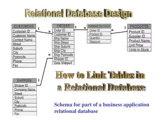
10.3.2 3NF decomposition algorithm(cont) Example 6:(From Desai 6.31) Beginning again with the SHIPPING relation. The functional dependencies already form a canonical cover. • From Ship→Capacity, derive R1(Ship,Capacity), • From {Ship,Date} → Cargo, derive R2(Ship , Date , Cargo), • From {Capacity,Cargo} → Value, derive R3(Capacity , Cargo , Value). • There are no attributes not yet included and the original key {Ship,Date} is included in R2.
10.3.2 3NF decomposition algorithm(cont) Example 7: Apply the algorithm to the LOTS example given earlier. A minimal cover is { Property_Id→Lot_No, Property_Id→ Area, {City,Lot_No} →Property_Id, Area → Price, Area → City, City → Tax_Rate}. This gives the decomposition: R1 (Property_Id, Lot_No, Area) R2 (City , Lot_No, Property_Id) R3 (Area, Price , City) R4 (City, Tax_Rate) Exercise 1: Check that this is a lossless, dependency preserving decomposition into 3NF. Exercise 2: Develop an algorithm for computing a key of a table R with respect to a given F of FDs.
Summary • Data redundancies are undesirable as they create the potential for update anomalies, • One way to remove such redundancies is to normalisea design, guided by FD’s. • BCNF removes all redundancies due to FD’s, but a dependency preserving decomposition cannot always be found, • A dependency preserving, lossless decomposition into 3NF can always be found, but some redundancies may remain, • Even where a dependency preserving, lossless decomposition that removes all redundancies can be found, it may not be possible, for efficiency reasons, to remove all redundancies.