Lectures 1 & 2: Basic Image Analysis
Learn the fundamentals of basic image analysis, including image representation, grey-level processing, and neighbourhood processing. Explore applications in microscopy, material analysis, and industrial inspection.

Lectures 1 & 2: Basic Image Analysis
E N D
Presentation Transcript
Lectures 1 & 2:Basic Image Analysis Dr Carole Twining Thursday 18th March 10:00am – 12:00am
Basic Image Analysis • Limited to simple 2D scenes • Adequately described as background and objects • Good contrast between objects and background • staining or backlighting • Constrained applications • microscopic materials analysis • biomedical microscopy • industrial inspection
Sample Problem: • Stained preparation, light microscope • Chromosomes, with bands • Measure banding pattern
Solving the Problem Questions Plan What is an image? Distinguish between objects & background What is background? Locate each individual object From not-background to distinct objects Locate centerline Shape of an object? Measurements on object Measure bands
Overview: • Image Representation • What is an image? • Grey-Level Processing • Improving the starting image • Segmentation • Background pixels and object pixels • Binary Image Processing • Improved background/object binary image • Measurement • Object as connected region
Image Representation • Isn’t it totally obvious? We all know what an image is! • Various ways of representing an image, depending on the task in hand • Image function • Landscape • Array of pixels • Image histogram • In another space entirely!
Image Image Plane x x y y Image Function Image Landscape brightness becomes height Image Representation
Zoom Image Representation Array of Pixels: Values and spatial relationship
Image Representation • Sort pixels by grayscale value/colour and stack them up Image histogram: Kept values but lost spatial information
Image Representation • Fourier Analysis: • any signal can be decomposed into a sum of sinusoids (FFT) • low frequencies, general shape, high frequencies details zero frequency at centre NOTE: zero frequency removed by subtracting mean value across image from image before doing FFT
NOTE: Image Representation • Frequency Space: • Integrate over the image, weighted by complex exponentials • Compact vector form: • Inverse:
Grey-Level Processing • Restoration: • What is noise, what is signal? • Remove blurring • Enhancement • Emphasize required features (e.g., linear features) • Emphasize change (e.g., surveillance)
Grey-Level Processing: Overview • Point processes • Transform global gray-level scale • Neighbourhood Processing • Values and their context • Image Arithmetic • Using a sequence/pair of images • Image Transforms • Images in a different space (frequency space)
position new pixel value pixel value function Grey-Level Processing: Point Processing • Point = Pixel • Transforms image based on single pixel value alone: • Various choices for monotonic function f(i) • Increase/decrease/stretch brightness and contrast • Gamma correction, power law : • Histogram matching between images • Histogram equalization
Re-assign colours, keep ordering (light to dark) Increase contrast Image Histogram Point Processing: Histogram Equalisation uneven distribution
Neighbourhood Processing single black pixel • Consider a single pixel value in context of neighbours • Neighbourhood (e.g. 3 x 3), structuring element (SE) • Two methods: • Convolution • Rank Filtering Noisy dark area Just noise
Same grayscale value MASK Aside: Context in Human Vision
1 2 1 1 0.5 1 1 0.5 0.5 0.5 1 1 1 0.5 0.9 0.9 0.6 0.5 0.6 0.9 1 Normalize the weights Convolution: 1D Example NOTE: 0 black to 1 white 0 to 255 8-bit images • Weighted sum of neighbours 0 0.37
g(-1,1) g(0,1) g(1,1) g(-1,0) g(0,0) g(1,0) g(-1,-1) g(0,-1) g(1,-1) Normalize the weights Convolution: 2D X g(a,b)
Convolution: 2D • Asterisk notation: • Discrete form: • Integral form: • Integral form (vector notation)
Convolution: Common Kernels • Gaussian: • Smoothing kernel • Any unimodal kernel smoothes the image • Difference of Gaussian (DoG) • Laplacian (or Laplacian of Gaussian) • similar shape to DoG, second-derivative filter • First-derivative edge filters • ridges at edge positions
NOTE: Convolution Theorem • Frequency space (see Image Representation) : • Look at it in frequency space or real space: • convolution in real space ,multiplication in frequency space • convolution in frequency space , multiplication in real space
0 100 0 Convolution Theorem: Gaussian Real space Frequency space
signal at edges 0 Convolution Theorem: Difference of Gaussians • band-pass filter, enhances edges • Laplacian and LoG similar
Gaussian and FT of Gaussian Convolution Theorem Gaussian Laplacian Inverse FT FT of Image Convolution with Gaussian, parameter Convolution Theorem: Laplacian of Gaussian & Difference of Gaussians • Do the derivative: • LoG: difference of infinitesimally-separated gaussians • DoG: difference of finitely-separated gaussians Laplacian of gaussian:
3x3 mean 3x3 median Noisy Image Neighbourhood Processing: Rank Filtering • Output is rank function of neighbourhood: • median (smoothes and preserves edges) • max and/or min (mathematical morphology) • rank number (seven of nine) • Harder to analyse than convolution
Mean: 2/3 + 1/3 = 1/3 + 2/3 = Median: 6 & 3 => 6 & 3 => X Rank Filtering & Edges: Example 3x3 SE
Original maximum 7th of nine Neighbourhood Processing: Rank Filtering • Rank Number • 3 x 3 structure element blocky, impressionistic effect
Original Addition Noisy 1 Noisy 2 Image Arithmetic: Addition • Take average over images in sequence • Reduces noise
Image Arithmetic: Subtraction • Take difference: • Negative values? Shift and scale to get back to [0:255] • Or take absolute difference • Static background, detects change • Object, shadows & reflections in real-world scenes
Image Arithmetic: Subtraction • Digital subtraction angiography (DSA) • Pre-study radiograph • Contrast agent injection • Post-contrast radiograph • Difference
Segmentation: Task: label each pixel as either object or background • Grayscale image → binary label image • Thresholding • simple, high-contrast images • Adaptive thresholding • simple images with shaded background • Advanced Segmentation • open research problem
Thresholding Adaptive Thresholding Segmentation: Thresholding profile
Threshold 100 Threshold 110 Threshold 140 Segmentation: Thresholding • Varying the Threshold • Need to choose threshold with care, • How to improve the binary image
Segmentation: Adaptive Thresholding Original Image Background corrected Smoothing Subtract Threshold Threshold Estimate of varying background Adaptive thresholding works provided you can obtain reasonable estimate of background shading
Binary Processing Aim: Improved binary image • Restoration or enhancement • Neighbourhood Processing: • binary morphology (erosion & dilation) • skeletonization • Image Logic: • combining binary images for more complicated processing
Binary Morphology: Erosion • Structure element (example, centre marked): • Binary object: • Sweep SE along boundary, and delete region covered
Binary Morphology: Dilation • Structure element (centre marked): • Binary object: • Reverse of erosion • Sweep SE along boundary, and add region covered Erosion + Dilation Rounded-off the corners
Binary Morphology: Dilation, Implementation via Neighbourhood Processing • Pixellated structuring element • Pixellated image object • Scan SE over image, and add pixel at defined centre if any object pixel lies within SE • Object erosion is dilation of background, so similar