Download
1 / 53
530 likes | 554 Views
Learn about the Solar-B mission's instruments - EUV Imaging Spectrometer (EIS), Solar Optical Telescope (SOT), X-Ray Telescope (XRT) - and its priority science plan. Explore mechanisms heating the corona, magnetic flux tubes, and energy transfer in the quiet Sun.

E N D
The Solar-B Mission Len Culhane – EIS Principal Investigator Louise Harra – UK EIS Project Scientist Mullard Space Science Laboratory University College London
SUMMARY • The Solar-B mission is outlined and the instruments described – EUV Imaging Spectrometer (EIS) in more detail • Solar-B mission operations are described • proposal submission is discussed • EIS planning software is summarized • possible joint observations with other missions suggested • The Solar-B priority science plan for the first 90 days after commissioning is reviewed
EIS - MSSL/NRL/BIRM/RAL → EUV Imaging Spectrometer SOT - ISAS/NAOJ → Solar Optical Telescope XRT - SAO/ISAS → X-ray Telescope FPP - Lockheed/NAOJ → Focal Plane Package SOT EIS FPP XRT Solar-B Spacecraft EIS – UiO → QL Software ESA/NORWAY → Svalbard Ground Station
Mission Characteristics • Launch date: 23rd September, 2006 • Launch vehicle: ISAS MV • Mission lifetime: 3 years • Orbit: Polar, Sun Synchronous • Inclination: 97.9o • Altitude: 610 km. • Mass: 900 kg • Mission control: ISAS/Uchinoua • Data downlink: • Uchinoura → 4 orbits/day • Svalbard → 15 orbits/day
Solar-B Science Summary • Establish the mechanisms responsible for heating the corona in active regions and the quiet Sun • Active region evolution • Nature of sub-photospheric magnetic flux tubes • Upper atmosphere heating and wave energy • Determine the mechanisms responsible for transient phenomena, such as flares and coronal mass ejections • Flares and the role of magnetic reconnection • Photospheric magnetic field helicity and CMEs • Investigate the processes responsible for energy transfer in the quiet Sun • Origin and nature of quiet Sun magnetic fields • Flux cancellation and ephemeral regions • Network and weak internetwork magnetic fields
Solar-B Mission Instruments • Solar Optical Telescope (SOT) Largest optical telescope (d = 0.5m) to observe Sun from space Diffraction-limited (0.2 – 0.3 arc sec) imaging in range 3880 – 6680 Å Vector magnetic field and velocity measurement at the photosphere • X-Ray Telescope (XRT) High angular resolution ( < 2 arc sec) coronal imaging Wide temperature coverage: 1 MK < Te < 30 MK • EUV Imaging Spectrometer (EIS) Coronal raster imaging at 2 arc sec Plasma diagnostics (Te, ne, v) in 170 – 210Å and 250 – 290Å ranges
Secondary Primary CLU Tip Tilt Mirror FPP Optical Component Layout Littrow Mirror Folding Mirror 448 x 1024 CCD X3 Mag lens Polarizing BS Scanning Mirror Folding Mirror Shutter Slit Field lens Grating Field lens Preslit X2 Mag lens Shutter 2048 x 4096 CCD Filterwheel Birefringent Filter FieldMask Telecentric lenses Beam Distributor Filterwheel 50 x 50 CCD OTA CommonOptics CT NFI BFI SP Folding Mirror Reimaging Lens Demag lens Image Offset Prisms Folding Mirror Polarization Modulator
Filtergraph Fields of View • Rectangle shows the Narrowband Filter FOV, 320 x 160 arc • sec with 0.08 arc sec pixels (4096 x 2048) • - inner square is 160 x 160 arc sec • Broadband Filter system • has higher magnification • (0.053 arc sec pixels) to • preserve SOT diffraction- • limited resolution • Broadband Filter FOV is • 216 x 108 arc sec • Both filter systems share • a single CCD.
Filtergraph Observables • Filtergrams • Broad-band Filter Imager: all 6 bands - only observable made by BFI • Narrow-band Filter Imager: all 9 lines and nearby continuum • Dopplergrams • Images Doppler shift of a spectral line - line of sight velocity • Longitudinal Magnetograms • Location, polarity and estimate of flux of magnetic field components along the line-of-sight • Stokes Parameters I, Q, U, V • Analysis of I, Q, U, V at multiple wavelengths in a spectral line yields vector magnetic field measurements → vector magnetograms, also from spectropolarimeter
Solar-B X-ray Telescope (XRT) Schematic • Grazing incidence telescope; average glancing angle 0.9o • PSF and detector pixel sizes are ~ 1 arc sec • – resolution ~ x 2.5 • better than Yohkoh • SXT • Ageom is 3.3 cm2 • Focal length is 2.7m • Inner diameter is 35cm • CCD (2k x 2k) gives • full-sun (33”) images • Focus adjustment for • optimum on-axis or • wide field resolution
X-ray Telescope Response • Telescope has ~ three times greater effective area than Yohkoh SXT • Nine filters cover 1MK < Te < 30 MKwith Te resolution D (log Te) = 0.2 • White light (G-band) solar images can be registered on the CCD at one filter • wheel position; allows X-ray and EIS to visible image alignment • XRT full-Sun observables: • → 33 arc sec X-ray & white light images
EIT and TRACE - EUV Coronal Images • Impact of better XRT resolution is • shown in a comparison of SOHO EIT • and TRACE EUV images • Resolution of XRT betters that of the • Yohkoh SXT by the same margin (x 2.5) • as a) TRACE images better b) EIT images • The SXT and TRACE images shown are • on the same scale and are of the same • coronal structures • In full-disk mode, the effective resolution • improvement over Yohkoh SXT is ~ x 5 b a
EIS - Instrument Features • Large Effective Area in two EUV bands:170-210 Å and 250-290 Å • Multi-layer Mirror (15 cm dia ) and Grating; both with matching optimized Mo/Si Coatings • CCD camera; Two 2048 (l) x 1024 high QE back illuminated CCDs • Spatial resolution: 1 arc sec pixels/2 arc sec resolution • Line spectroscopy with ~ 25 km/s pixel sampling • Field of View: • Raster: 6 arc min × 8.5 arc min; • FOV centre moveable E – W by ± 15 arc min • Wide temperature coverage: log T = 4.7, 5.4, 6.0 - 7.3 K • Simultaneous observation of up to 25 lines
Primary Mirror Entrance Filter CCD Camera Front Baffle Grating EIS Optical Diagram
Slit and Slot Interchange • Four slit/slot selections available • EUV line spectroscopy - Slits - 1 arc sec 512 arc sec slit - best spectral resolution - 2 arc sec 512 arc sec slit - higher throughput • EUV Imaging – Slots - Velocity information overlapped - 40 arc sec 512 arc sec slot - imaging with little overlap - 250 arc sec 512 arc sec slot - detecting transient events
Strong Isolated Lines for 40 arc sec Slot Imaging Short Wavelength Band Ionl (Å) Fe XI 188.2 Fe XXIV 192.0 Ca XVII 192.8 Fe XII 195.1 Fe XIII 202.0 Fe XIII 203.8 Long Wavelength Band Ionl (Å) Fe XXIV 255.1 He II 256.3 Fe XVI 263.0 Fe XIV 270.5 Fe XIV 274.2 Fe XV 284.1
Shift of FOV center with coarse-mirror motion Maximum FOV for raster observation 360 900 900 512 512 512 Raster-scan range 250 slot 40 slot EIS Slit EIS Field-of-View
EIS Effective Area Primary and Grating: Measured - flight model data used Filters: Measured - flight entrance and rear filters CCD QE: Measured - engineering model data used Following the instrument end-to-end calibration to ± 25%, analysis suggests that above data are representative of the flight instrument
w Science Observables • Observation of single lines • Line intensity and profile • Line shift ()→ Doppler motion • Line width (w) and temperature → Nonthermal motion • Observation of line pair ratios • Temperature • Density • Observation of multiple lines • Differential emission measure
EIS Sensitivity Detected photons per 11 per 1 sec exposure
a) b) SOT/FPP Data c) Solar-B Mission Data Acquisition • Data are stored on-board in 8 Gbit memory • Instrument memory allocations are: • - SOT/FPP → 70% • - EIS/XRT → 15% each • Data downlinked to Svalbard ground • station (ESA/Norway) on 15 orbits/day • - memory dumped once per orbit • EIS average data rate → 45 kbps • Command uplinks only from Uchinoura • - four memory dumps per day • Quick-look assessed at ISAS and Uchinoura
Level - 0 Reformat Solar - B Database in Japan FPP Level - 1 and -2 Reformat at Lockheed Level-0 and Cal Data Level-2 Data (FPP) Solar - B Database Solar - B Database in US in UK Solar-B Mission Data Distribution • Data distributed to UK, US and • Norway in compressed level – 0 • form • Because of complexity, FPP • data are transmitted in level – 0 • form to Lockheed Palo Alto • They are processed to level – 2 • to produce vector and scalar • magnetograms • These products are then sent • to Japan and onward to UK • and Norway
Solar-B Mission Operations • Mission operations will be conducted • from the ISAS Spacecraft Operations • Centre in Fuchinobe, Japan • Solar-B team observing plans and • community proposals will be discussed • at monthly meetings • Each instrument team will have a • Scientific Schedule Coordinator who will • organize the preparation of instrument • proposals and their integration in the • overall mission observing plan • Weekly and daily planning meetings • allow flexibility to respond to changing • solar conditions
Operations Roles A) Solar-B Mission • Solar-B Chief Planner (CP) • Provided by the instrument teams in rotation, one week shifts • Chief Planner Assistant (CPA) • Provided by the instrument teams in rotation, one week shifts • Scientific Schedule Coordinators (SSC) • One for each instrument • Assistance from other participating countries • EIS SSC based in MSSL with visits to Japan B) Individual Instruments (EIS-specific Roles) • Chief Observers (CO) (SOT, XRT, EIS): • One person for each instrument, one week shifts • Instrument Software Coordinators (ISCO): • EIS person initially at ISAS, then at MSSL; planning software from RAL • Instrument System Engineers (ISE): • EIS person at ISAS for commissioning, then at MSSL
Landi/Warren MSSL (x5) Mariska RAL (x2) Doschek Norway (x2) GSFC/Davila GMU/Dere NAOJ (x2) Post Doc/ MSSL Post Doc/ Brooks ISAS On-Site (1 year) EIS Operations Staffing UK/Norway/Japan NRL Bradley Sun --------- Culhane Harra, Other UK Rainnie Young EIS Planner (Rotator @ 3 weeks each) Hansteen Wikstol ISAS Hara Watanabe ISAS On-Site (1 year) Williams First year of operation (Minimum)
EIS Planning Tool Software • Planning tool software is in SSW • Users will need to install the EIS SolarSoft tree • Study Definition • Line Lists • Raster Definition • Study Definition • Planners then export studies to ASCII format • E-mail a formatted file and a science case to a dedicated account at MSSL
SOT Initial Science Plan • Active region tracking: - Emerging AR - Mature/decaying AR - Flaring AR - Subsurface flows - MHD waves • Quiet Sun: - Network flux dynamics - Internetwork flux - Convective flow structure • Irradiance: - Activity belt - Polar regions • Prominences/Filaments - Prominence at limb/Filaments on disc - Track boundary evolution
XRT Initial Science Plan • Flares fromdynamic AR on disk: Follow AR across disk, flare program loaded - Deploy range of filters and FoV sizes - Flare topology and energetics • Track modest (emerging or decaying) active region on disc: Image with large, medium and small FoVs - Structure, energetics and dynamic behaviour - AR evolution; track centre to limb? • Quiet Sun/X-ray Bright Points: Multi-filter study of bright points - Thermal structure and dynamics - Life-cycle statistics • Quiet Sun/coronal holes Single filter for boundary imaging - Track boundary evolution • Quiet Sun/filament Magnetic structure around filament - Track filament for 1-2 days
EIS Initial Science Plan • Flare trigger and dynamics: Spatial determination of evaporation and turbulence in a flare - Characterize AR topology - Measure key structures in detail - Flare trigger response for early velocity measurement • Active region heating: Spatial determination of v, Te and ne in active region structures - High time cadence sit and stare observations; dynamics - Observe AR global changes - Velocity measurements (± 3 km/s) • Quiet Sun and coronal hole boundary: Correlate coronal Te, ne and v with magnetic topology - Study corona above two supergranule cells - Study corona above bright point or explosive event - Observe above a coronal hole boundary • Quiet Sun and Prominences (assume no available AR) Spatial determination of v, Te and ne in surrounding regions -Register and follow eruption
EIS Core Science Programme • AR Heating → dynamic phenomena in loops • Coronal/Photospheric velocity field comparison in AR • Coronal Seismology → waves in AR structures • AR Helicity content → CMEs, magnetic clouds • Evolution of trans-equatorial Loops • Flare produced plasma → source, location and triggering • Flare reconnection → inflow and outflow • Quiet Sun transient events → network, network boundaries, CH boundaries, size scales • CME Onsets → dimming, filaments, flux-ropes, flaring AR, trans-equatorial Loops • Evolution of large coronal structures → streamers, large-scale reconnection, slow Solar Wind
Some Possible Joint Observations • Solar-B Instruments: • Active Region study campaign (SOT/EIS/XRT) • Emission measure distributions in AR structures (EIS/XRT) • AR helicity content and CME launches (SOT/EIS/XRT) • Magnetic topologies in small events (SOT/EIS/XRT) • Network and intra-network small event energies and velocities (EIS/SOT) • Plasma and magnetic structures above Coronal Hole boundaries (EIS/SOT) • Reconnection flows in flares (EIS/XRT) • Other Missions: • CME launching, topology and magnetic clouds (Solar-B, STEREO, ACE) • CME dimming outflow velocities; their relation to CMEs (Solar-B/EIS, STEREO) • Trans-equatorial loop and filament eruptions (Solar-B/EIS, XRT, STEREO) • Coronal (EIT) waves and their relation to CMEs (Solar-B/EIS, XRT, STEREO) • Intensity and velocity studies of waves in AR structures (Solar-B, TRACE, SDO) • Impulsive flares andsub-surface wave propagation (Solar-B, TRACE, SDO)
Processed Science Data Products • Intensity Maps (Te, ne): – images of region being rastered from the zeroth moments of strongest spectral lines • Doppler Shift Maps (Bulk Velocity): – images of region being rastered from first moments of the strongest spectral lines • Line Width Maps (Non-thermal Velocity): – images of region being rastered from second moments of the strongest spectral lines
EIS Data Flow Data compression DPCM(loss less) or 12bit-JPEG Small spectral window (25 max) CCD Readout Electronics 2Mbps max 1.3 Mbps EIS ICU S/C MDP control Observation table 250 kbps max for short duration, 45 kbps average Large hardware CCD window Average rate depends on number of downlink station. 1 slit obs. 40 slot obs. 250 slot obs. Spec.width 16 40 250 Spatial width 256" 512" 256" No. of lines 8 4 4 Compression 20% 20 % 20% Cadence 2 sec 5 sec 15 sec Rate 38.4 kbps 38.4 kbps 40 kbps Telemetry data format 10 min cadence for 44 rastering
Dual CCD Camera Grating Primary Mirror EIS Instrument Completed Filter Holder Installed Entrance Filter Holder Installation of Key Subsystems in Structure
Vector Magnetograms • Spectra of two Fe lines at 6301.5 Åand 6302.5 Å and nearby continuum are • exposed with a 0.16 x 164 arcsecond slit • The Spectro-polarimeter (SP) can scan across a 160 x 320 arc sec FOV while • the CT and Filter FOVs are fixed • In normal mode, the SP scans • 160 arc sec in 83 min • Fast maps are 2.8 times quicker • hence 160 arc sec in 30 min • Magnetic field measurement: • - B (longitudinal) to ± 3 G • - B (transverse) to ± 30 G • - Field direction to ± 1o
Velocity MeasurementAccuracy Flare line Bright AR line Photons (11 area)-1 sec-1 Photons (11 area)-1 (10sec)-1 Doppler velocity Line width Number of detected photons
EIS and XRT Science • Coronal heating mechanisms • - Multi-filter XRT and multi-line EIS slot images study thermodynamic properties ofcoronal structures • EIS and XRT can show the AR coronal structures that have significant large scale flows • Rapid intensity fluctuations observed by XRT combined with velocity maps from EIS and SOT Dopplergrams will • establish role of waves and flows in different parts of an AR • Magnetic reconnection and coronal dynamics • XRT will observe statistically significant numbers of small reconnection events • Comparing location, energetics, and duration of these events (XRT, EIS, and SOT filtergrams) with evolving • photospheric magnetic field will allow first quantitative study of • - conditions necessary for reconnection • - efficiency of the reconnection • - coronal impact of the reconnection • Photospheric-coronal coupling • For ARs, need to trace magnetic connectivity → photosphere – chromosphere -corona • Spectral imaging with EIS and SOT • - allows identification of loop footpoints • - associates footpoints with photospheric magnetic features • Flare events and coronal mass ejections. • Topological properties of flares and CMEs studied using non-linear force-free field models from SOT vector data • - Follow AR evolution and identify the coronal sites of flare or CME initiation • - Discover magnetic null points above flaring active regions and track AR magnetic helicity changes
EIS Instrument Calibration • If flin photons cm-2 s-1 sr-1 is the intensity of the solar radiation at wavelength • l, the number of photons registered in each detector pixel per second is: • Nl = flA wd Tffa(l) Tspider Rm(l) Tsef(l) Eg(l) Ed(l) where • A is the mirror geometric area and wd is the solid angle per detector pixel • Tspider is the transmission of the entrance filter spider support structure • Tffa(l), Tsef(l) are the transmissions of the Al entrance and spectrometer filters • - filters on an 85% transmission support mesh which is included in T values • Rm(l), Eg(l) are the coated mirror and grating efficiencies • Ed(l) is the CCD detector quantum efficiency
EIS Calibration Spectra – 250" Slit • Calibration has been carried out with the source • used for SOHO CDS calibration • (Hollandt et al., 2002, Lang et al., 2000) • Source is radiometrically calibrated by PTB, Berlin • at the BESSY I electron storage ring • Stable high-current hollow-cathode discharge lamp • provides appropriate EUV emission lines • Following EIS calibration, the source will be re- • calibrated at BESSY II • NRL Penning source also used for alignment and full • aperture illumination
Al III, Al IV and Ne IV lines EIS Calibration Spectrum – 2" Slit
Nonthermal Velocity in Flares Te • Gradual increase of vnt at the precursor phase of a flare is reported by Harra, Matthews, & Culhane (2001). • Detecting of flares in a slit scanning observation is the only way to identify this precursor. • Identification of site of large non-thermal velocity in imaging spectroscopy will be very important in understanding the physics of precursor phase. vnt vnt I (S XV) vnt BATSE Ch 1 Harra, Mattews, & Culhane 2001, Ap.J, 549, L245-248
Reconnection Inflow • Evidence of 2D-reconnection inflow for a long-duration event is reported by Yokoyama et al. (2001) from an EUV imaging observation • EIS will detect the reconnection inflow as a Doppler shift in emission line spectra • Observation near the limb will be important to detect reconnection inflow • Hot reconnection outflow may be detected in Fe XXIV slot observations Movie sequence From Yokoyama et al. 2001, ApJ, 546, L69-72