Download

1 / 28
280 likes | 294 Views
A comprehensive system for managing the Elbe River floodplains, incorporating aims like flood protection, water management, agriculture, and tourism through an AI-based approach. Utilizes case-based reasoning, ontology, and qualitative reasoning to make informed decisions.

E N D
Intelligent decision support system for riverfloodplain managementPeter Wriggers, Marina Kultsova, Alexander Kapysh, Anton Kultsov, Irina ZhukovaLeibniz University Hannover, Hannover, Germany, Volgograd State Technical University, Volgograd, Russia,
BiosphereReserve Elbe River Landscape in Lower Saxony More then 20 stakeholders: • Administration of the Elbe river biosphere reserve (ABRE); • Environmental Ministry of Lower Saxony; • District of Lueneburg (Water Department, Nature Conservation Department); • District of Luechow-Dannenberg (Water Department, Nature Conservation Department); • Municipalities with areas in the Elbe floodplains; • Water Management and Flood Control Authority; • Dike Associations; • Disaster Control Authority; • Water and Soil Associations; • Agricultural Ministry, Chamber and Associations of Lower Saxony; • Fishing Associations and Companies; • Nature Conservation Associations; • Ministry of Economy of Lower Saxony; • Tourist Associations and Companies; • Administrations for Waterways and Navigation; • Navigation companies. The Elbe Riverland covers the area within the borders of the UNESCO Biosphere Reserve Elbe River Landscape in Lower Saxony reaching from Elbe-km 472.5 near Schnackenburg to Elbe-km 569 near Lauenburg. Altitude varies from 5 to 109 m NN. The overall area of the biosphere reserve comprises some 56,760 hectares.
Identification of aims, subaims and attributes Global aim: Conservation and development of the Elbe river floodplains in a state, that the claims of water management, flood protection, agriculture, fishery, nature conservation, tourism and navigation are answered at the best possible rate. Priorities: Aspects: • Flood protection; • Water management; • Agriculture; • Fishery; • Nature conservation / ecology; • Tourism; • Navigation. 1st priority Flood protection in case of extreme flood events if life or properties of people are acutely threatened
Description of a decision making problem has a complex and variable structure; Components of the problem and solution descriptions can significantly differ in their importance; There are multiple logical relations between components of problem description; Both qualitative and quantitative parameters, which should be interpreted in a context-dependent way (not by absolute value), are taken into account; Knowledge about previously solved problems which are similar to the current one is actively used while decision making. Domain knowledge features
Concept of CBR-based decision making (I) • Appropriate AI technologies for the intelligent decision making in floodplain management: ontological knowledge representation model, case based reasoning and qualitative reasoning. • While CBR is a leading reasoning mechanism, QR and ontology carry out the knowledge-based support of the main stages of CBR. • CBR process is strongly supported with ontology and qualitative reasoning at all stages, such "knowledge-intensive"approach allows to improve the accuracy and correctness of the obtained CBR solutions.
Concept of CBR-based decision making (II) • Ontology defines case representation model and sets of parameters for case description with their possible values. Ontology contains information about the aims of stakeholders, aim attributes and their possible values. Ontology defines foundation for case description, and it can be used as a knowledge base for subsystem of automated case formulation; • If the user has dened case index incompletely, ontology can be applied at the stage of case retrieval for redenition of the case. Also the algorithm of similarity measure calculation depends heavily on the case representation model, which is defined by ontology; • Ontology is used at the stage of case adaptation to make decision about alternative values of parameters if adaptation algorithm has proposed a few equivalent choices, for example, a few possible values for one attribute; • Ontology contains qualitative model of case and consistency rules which can be used at the stage of case revision. Consistency rules dene infeasible combinations of parameter values for dierent aspects of case description.
General schema of integration of CBR, QR and ontology Ontology Query generation Case representation model 1 Case retrieval Domain knowledge 2 Case adaptation 3 Casebase 4 Case revision Case qualitativemodel 5 Case retention 1 - case structure, 2 - formalized domain knowledge, 3 - stored case, 4 - new case, 5 - qualitative simulation results.
Modied CBR-cycle supported with QR and ontology 1 - problem description, 2 - CBR-query, 3 - case index, 4 — retrieved cases, 5 - adapted solution, 6 - revised solution, 7 - new case, 8 - case structure, 9 - stored cases, 10 - expert rules, 11 - adaptation rules, 12 - consistency rules, 13 - qualitative simulation results, 14 - domain conceptualization, 15 - case descriptions, 16 - general domain knowledge, 17 - qualitative dependencies between components of case description.
Ontological knowledge representation model ONT =< DO;CS;QM >; (1) where DO { domain ontology, CS { case structure, QM { case qualitative model. DO = fOB; ATT;DAT;ACT;CR;AR;QD;RELg; (2) where OB = fOB1;OB2; :::;OBng { set of stakeholders' objectives; ATT = fATT1 [ ATT2 [ ::: [ ATTng { set of attributes which are used for problem description, each subset ATTi corresponds to objective OBi; DAT { set of ontology domains, which dene the space of attribute values; CR { set of consistency rules; AR { set of adaptation rules; ACT = fACT1 [ ACT2 [ ::: [ ACTng { set of actions, each subset ACTi corresponds to objective OBi; QD { set of qualitative dependencies between attribute values, QD : ATT ATT ! fI+; I; P+; P;?g, where I+ { positive direct inuences, I { negative direct inuences, P+ { positive indirect inuences, P { negative indirect inuences; REL = fREL1;REL2; :::;RELkg { set of relations between ontology concepts.
Case representation model CS = fP; S(P);CRELg; (3) where P { problem description (also can be referred as a case index); S(P) { problem solution description as a set of actions which were applied; CREL = fCREL1;CREL2; :::;CREL8g { set of case relations. Set CREL contains the following relations: CREL1 { relation hasInitialState, CREL2 { relation hasActionSet, CREL3 { relation hasResultState, CREL4 { relation hasCausalState, CREL5 { relation hasEffectiveState, CREL6 { relation hasAssessmentSet, CREL7 { relation hasCertainAction, CREL8 { relation hasCertainAssessment.
Case qualitative model QM = fBBC;ACg; (8) where BBC { set of QM model primitives; AC { set of compound components composed of the primitives. BBC = fSB;BB;ABg; (9) where SB { set of structural primitives; BB { set of primitives describing behaviour of the model; AB { set of premises dening the applicability of compound components of model. SB = fSE; SCg; (10) where SE (OB [ ATT [ ACT) { entity hierarchy reecting the concept hierarchy of the problem domain; SC { set of relations between entities. BB = fQU;QS;Dg; where QU ATT { set of quantities; QS DAT { set of quantity spaces; D QD { set of causal relations between quantities, D has the following range of values fI+; I; P+; Pg. AC = fSF; PF; SCg; (12) where SF { set of static model fragments; PF { set of process model fragments; SC { set of simulation scenarios.
Reasoning mechanism The following algorithms were developed to operate on the suggested ontological knowledge representation model in the framework of the CBR mechanism implementation: • CBR-query formulation support algorithm which allows reducing the amount of the routine work needed to input information and enforcing knowledge representation model integrity as well as redening the case index with use of general domain knowledge in form of DL rules.; • Case retrieval algorithm which uses class (concept)-based similarity (CBS) computation algorithm and property (slot)-based similarity (SBS) computation algorithm; • Case adaptation algorithm which uses domain knowledge in form of DL rules; • Case revising algorithm which uses the results of qualitative simulation on the case qualitative model.
ПОИСК ПРЕЦЕДЕНТОВМера близости Общая мера близости: Мера близости дескрипторов интервального типа: Мера близости дескрипторов типа «дата»: Мера близости дескрипторов вещественного типа: Мера близости дескрипторов типа «перечисление»: 17
МЕРА БЛИЗОСТИ прецедентов CBS, SBS Для оценки меры близости дескрипторов, представляющих собой качественную переменную или таксономию применяется алгоритм оценки близости экземпляров онтологий на основе анализа иерархии классов онтологии: Алгоритм SBS (slot based similarity) предназначен для поискамеры близости между двумя прецедентами с учетом объектных отношений между компонентами описания прецедента в виде отношений онтологии и представляет собой рекурсивную функцию обхода графа, в котором узлами являются концепты онтологии, а дугами – объектные отношения онтологии: Предлагаемый алгоритм SBS отличается от известного тем, что позволяет учесть разницу в описании между прецедентом из базы прецедентов и запросом. 18
ПОКАЗАТЕЛЬ ЭФФЕКТИВНОСТИ для алгоритма поиска прецедентов Для каждого прецедента в базе прецедентов доступно описание конечной ситуации, которая сложилась после применения указанных в прецеденте мер воздействия к начальной ситуации. Разницу в оценках начальной и конечной ситуаций прецедента предлагается использовать как показатель эффективности E, который позволяет оценить степень полезности решения рассматриваемого прецедента к РПП-запросу Q где: E – показатель эффективности, A – оценка начальной ситуации по i-му аспекту, – оценка конечной ситуации по i-му аспекту, diff – разница между оценками, W – весовой коэффициент i-го аспекта, N – количество аспектов. 19
Case retrieval algorithm 1. Define preferences of decision maker PREFi and weighting factors WAi ; 2. Compute Sim and E for each case Cj from case base CB; 3. Form empty result vector SC: SCj = (Cj ; vj ), where vj - condence factor for Cj ; 4. Form set of cases Cp for which 8Cj 2 CP : Sim (Cj ;Q) > SimMIN \ E (Cj ;Q) > 0, where SimMIN = min Cj2CB Sim (Cj ;Q); 5. Add to list SC not more then M pairs (Cj ; vj ), for which Cj : Cj 2 CP \ E (Cj) = EMAX, state vj = E (Cj ); 6. Add to list SC not more then M pairs (Cj ; vj ), for which Cj : Cj 2 CP \ Sim (Cj ;Q) = SimMAX, state vj = SIM (Cj ;Q). Vector SC is the output of retrieve algorithm.
Case adaptation algorithm 1. Form empty list AcSC of pairs fAc; vag where Ac - action, va - condence factor; 2. For each pair fCj ; vjg from SC do: (a) For each action Aci from Cj add pair fAci; vjg to AcSC list (i.e. add actions from retrieved cases with condence factor v); 3. Perform reasoning on ontology; 4. For each action AcR inferred in accordance with adaptation rules, add pair fAcR; 1g to AcSC list; 5. If list AcSC is empty, when case base and ontology is not applicable to current DSS-query, adaptation is unsuccessful; otherwise 6. Sort list AcSC by descendant of condence factor va; 7. Remove incongruous actions from AcSC list: (a) Set i = 0; (b) For each jAcSCj > j > i remove pair fAcj ; vag from AcSC if MIij = 1; (c) Set i = i + 1; (d) If jAcSCj > i then go to step (b) 8. Form case solution list AcS that consists of actions Aci from list AcSC. The case solution list AcS is the output of adaptation algorithm.
Case revising algorithm 1. Generate new case C as an individual of "Case" class which has index Ind coincident with CBR-query Q and solution Acs; 2. Perform the procedure "classify taxonomy" on ontology; 3. If case C was classied as individual of "inconsistency" class (in accordance with consistency rules), then revision is unsuccessful, remove case C; 4. Simulate the qualitative model for case C and dene assessment A i for obtained result state; 5. Compute E(C) using (23); 6. If E(C) < 0, then revision is unsuccessful, remove case C; 7. If 0 6 E (C) < E, where E is average E-value for stored cases, then revision is quasi-successful, use solution Acs for current problem, but don't retain case C in case base; 8. If E (C) > E, then revision is successful, retain case C in case base.
jRamwass system architecture 1 - case structure, 2 - stored cases, 3 - domain knowledge in form of DL-rules, 4 - asserted and inferred knowledge, 5 - case qualitative model in OWL-format, 6 - case qualitative model in GARP3- format, 7 - redenition rules, 8 - adaptation rules, 9 - consistency rules, 10 - qualitative simulation results, 11 - problem description, 12 - CBR-query (case index), 13 - values of similarity measures, 14 - set of similar cases, 15 - adapted solution, 16 - new case.
Decision making process using IDSS jRamwass 1. Formalization of problem description { identifying the aim hierarchy, aim attributes and values, priorities of decision maker. 2. Formulation of CBR-query in framework of case representation model. 3. Redenition of CBR-query using inference on expert rules and generation of case index (description of problem situation). 4. Retrieve of the similar cases in case base using retrieve algorithm based on CBS and SBS similarity metrics. 5. Selection of the relevant cases for reuse. 6. Adaptation of the selected cases' solutions to the new problem using adaptation algorithm based on inference on adaptation rules. 7. Revision of the new adapted solution using simulation on case qualitative model and inference on consistency rules. 8. Generation of a new case for the solved problem in framework of case representation model. 9. Retention of the new case in the case base for further use.
Пример решения задачи управления с помощью системы. Описание запроса к системе. Создание рекреационной зоны • Предпочтения хозяйствующих субъектов: • Туристические компании: высокий приоритет • Экологи: средний приоритет • Остальные: низкий приоритет • Расположение территории: • 559-й километр реки Эльба • Левый берег • Параметры ситуации: • Площадь участка: 67 км. кв. • Строения: нет • Способ землепользования: лиг, низкотравье • Обзорность участка с дамбы: хорошая • Доступность воды: плохая • Количество обзорных точек: хорошо • Высота дамб: хорошо • Состояние дамб: хорошо • Колебание уровня воды: хорошо • Оценка начальной ситуации по аспектам: • Сельское хозяйство: хорошо • Рыболовство: удовлетворительно • Защита от наводнений: удовлетворительно • Судоходство: удовлетворительно • Затраты на обслуживание: удовлетворительно • Сохранение природы: хорошо • Туризм: удовлетворительно 25
Пример решения задачи управления с помощью системы. Получение решения. Результаты поиска Прецедентов Наиболее близкие прецеденты: • № 16 – преобразование участка в рекреационную зону • № 21 – сохранение луга • № 13 – перемещение дамб Трассировка процесса адаптации Результаты адаптации 26
ТЕСТИРОВАНИЕ СИСТЕМЫ Тестовая база составляет 42 прецедента; Совпадение результатов стандартного алгоритма с экспертным решением составляет в среднем 67%; Совпадение результатов предлагаемого алгоритма с экспертным решением составляет в среднем 88% , где NSOL – количество элементов решения прецедента С, N*SOL – количество элементов совпадающих элементов решения С и Сi 27