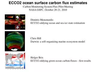
ECCO2 ocean surface carbon flux estimates Carbon Monitoring System Flux-Pilot Meeting

1. ECCO2 ocean surface carbon flux estimates Carbon Monitoring System Flux-Pilot Meeting Caltech, February 8, 2011 Dimitris Menemenlis ECCO2 eddying ocean and sea ice state estimation Chris Hill Darwin: a self-organizing marine ecosystem model Holger Brix ECCO2-Darwin carbon fluxes – towards equilibrium

2. ECCO2 Eddying global-ocean and sea-ice data synthesis for improved estimates and models of ocean carbon cycle, understanding recent evolution of polar oceans, monitoring time-evolving term balances within and between different components of the Earth system, and many more science applications. Velocity (m/s) At 15 m depth

3. Eddying, global-ocean, and sea ice solution obtained using the adjoint method to adjust ~109 control parameters Normalized cost for ARGO T Cost functions reduction during first 16 forward-adjoint iterations Normalized cost for ARGO S

4. Reduction of root-mean-square model-data residual rms(Optimized – AMSRE SST) – rms(Baseline – AMSRE SST) °C rms(Optimized – JASON SSH) – rms(Baseline – JASON SSH) m

5. JPL HolgerBrix DimitrisMenemenlis Hong Zhang MIT Stephanie Dutkiewicz, Mick Follows, Oliver Jahn, David Wang, Chris Hill Biogeochemical approach based on “self-organizing” principle – Follows et. al, Science, 2007. Darwin ecosystem model in ECCO2 cs510. environmental physiological 78 virtual species with different growth curves f(I,T,pH,…) Ecosystem Species abundance from 78 possible types in environment set by interplay between circulation, nutrients and physiology.

6. Conventional, ocean color, view of solution vsSeaWIFS Top panel – SeaWIFS monthly composite Chl concentration 1998-1999. Bottom panel – cube84 + 78 species self-organizing ecosystem model simulation for 1998-1999. i.e can recover fields that are calculated in traditional NPZD approach… but can now look at what species are contributing to Chl where and when.

7. Species mix v. space and time – global view. SeaWIFSChl comparison on previous slide is integral over multiple different species (both in real wolrd and in model). Movie shows concentration of different species categories as a function of space and time. Diatoms (red), prochlorococus (green), picoplankton(blue), everything else(yellow) all contribute to the overall growth rate. At different times at some location different species may dominate. This is driven by relative fitness of the species wrt to local nutrient, light, temperature conditions – but it is also modulated by fluid transport. Armstrong, Nature Geoscience, 2010.

8. Species mix v space and time – local views. Individual species abundance at yellow x as function of time. × Hofmuller plots of individual species abundance at point on white line. The plot and animation show views of abundance of individual species over time at an Eulerian point.

9. Can relate to ecological provinces. Model species abundance should be equivalent to “provinces” (Longhurst) – can be compared against observationally inferred provinces. Role of flow can be understood through looking at local growth rate versus actual abundance (which includes fluid transport). Biological “provinces”, M. Oliver et. al (derived from color + SST obs)

10. Connecting to CO2 estimates • cs510 + ecosystem  alternate perspective on biological activity, species diversity. • emergent virtual species analogs of ocean ecotypes. • for CMS nutrient source/sink terms include • carbon chemistry. • carbon exchange with organic pool for each species is function of growth/decay.  provide a time evolving physical and biological environment for air-sea CO2 flux estimates.  also get information on what “virtual species” categories take up and where and when for free! Follows et. al, Science, 2007.

11. ECCO2-Darwin Carbon FluxesTowards Equilibrium Holger Brix DimitrisMenemenlis, Chris Hill, Oliver Jahn, Stephanie Dutkiewicz, Mick Follows, David Wang

12. Air-sea fluxes: Mechanisms chemical exchange phyto2 phyto1 phyto3 phyton remineralize at depth…..

13. Spin-up of ECCO2-Darwin biogeochemical model Globally integrated air-sea CO2 flux (PgC/yr) positive: outgassing, negative: ocean uptake • Cycling with 2004 ECCO2 • ocean state estimate • pCO2atm = 370 ppm • spin-up until • global-mean CO2 flux << rms(CO2 flux) • then transition from 2004 to 2009 • with realistic pCO2atm 2.5 2.0 1.5 1 0.5 0 -0.5 -1 1 2 3 4 5 6 7 8 9 10 spin-up time (years)

14. ECCO2-Darwin sea-air CO2flux (10-9kgC/m2/sec)

15. Backup slides

16. 1.1±0.7 PgC y-1 4.1±0.1 PgC y-1 47% 2.4 PgC y-1 27% Calculated as the residual of all other flux components + 7.7±0.5 PgC y-1 26% 2.3±0.4 PgC y-1 Average of 5 models Fate of Anthropogenic CO2 Emissions (2000-2009) Global Carbon Project 2010; Updated from Le Quéré et al. 2009, Nature Geoscience; Canadell et al. 2007, PNAS

17. Globally integrated air-sea fluxes (PgC/yr) positive: outgassing, negative: ocean uptake 1 0.5 0 -0.5 -1 -1.5 -2 ECCO2 +0.4 PgC/yr • First comparison: • ECCO2 not yet taking up CO2 • Annual means of oceanic • uptake in models and • climatology is too small GSFC -0.7 PgC/yr Takahashi (-1.4 PgC/yr) 1 2 3 4 5 6 7 8 9 10 11 12 time (months)

18. Annual mean surface CO2 flux map (10-9kgC/m2/sec) 2 1.5 1 0.5 0 -0.5 -1 -1.5 -2 2 1.5 1 0.5 0 -0.5 -1 -1.5 -2 ECCO2-Darwin spin-up GSFC 2009/10 2 1.5 1 0.5 0 -0.5 -1 -1.5 -2 Takahashi Climatology