Download
1 / 45
450 likes | 641 Views
Designing the data warehouse / data mart. Methodologies and Techniques. Basic principles. Warehouse Database. Life cycle of the DW. First time load. Operational Databases. Refresh. Refresh. Purge or Archive. Refresh. Data transfers into a database. First time system implementation

E N D
Designing the data warehouse/ data mart Methodologies and Techniques
Warehouse Database Life cycle of the DW First time load Operational Databases Refresh Refresh Purge or Archive Refresh
Data transfers into a database • First time system implementation • From a manual system • Data warehousing projects • Database version upgrade • ERP projects • Migration • From old to new system
Data transfers between systems • Dynamic data (eg. sales orders) • Interface required? • Static data (eg. customers) • Conversion required?
What can go wrong • Data not available • feature activated from implementation onwards • Massive data entry • Eg: different account structure • Data incomplete • Data inconsistent (eg: engineering vs accounts) • Wrong level of granularity • Data not clean • New system requires changes – new product codes
Data cleaning must address • Different department record same info under different codes • Multiple records of same company (under different names) • Fields missing in input tables (eg: c/o) • Different depts. Record different addresses for same customer • Use of different units for time periods
Labour intensive tasks • Data entry • Data checks • Working on solving conflicts • Allocating new codes • Solution = introduce as much automation as possible • SQL / SQL loader (Oracle) • Custom conversion programmes to extract, modify and upload data • Filtering • Parsing (eg: excel) • Staging areas for conversion in progress
Data utilities • ORACLE is king of data handling • Export: to transfer data between DBs • Extract both table structure and data content into dump file • Import: corresponding facility • SQL*loader automatic import from a variety of file formats into DB files • Needs a control file
Control files: using SQLloader • Data tranfers in and out of DB can be automated using the loader • Create a data file with the data(!) • Create a control file to guide the operation • Load creates two files • Log file • “bad transactions” file • Also a discard file if control file has selection criteria in it
Example 1 – the supplier file New supplier code to include city where firm is based Assignation of category based on amounts purchased OLD Sup code Sup name Sup address City Phone 4 digits
Example 1 – the supplier file New supplier code to include city where firm is based Assignation of category based on amounts purchased OLD Sup code Sup name Sup address City Phone 4 digits NEW Sup code Sup name Sup address… Phone Cat 3 letters + 1,2,3 depending 4 digits on total purchases last year
Example 2 – New Cost Accounting Structure Maintenance department expenditure: 1 account => separate accounts for different production activities OLD Intervention code Desc. Date Labour Parts Total
Example 2 – New Cost Accounting Structure Maintenance department expenditure: 1 account => separate accounts for different production activities OLD Intervention code Desc. Date Labour Parts Total NEW Intervention code Desc. Date labour Parts Total Account
Example 3: merging files • Complete customer file based on Accounts and Sales and Shipping OLD (finance) CustID name address city account number credit limit balance OLD (sales) CustID* name address city discount rates sales_to_date rep_name OLD (Shipping) CustID** name address city Preferred haulier
Example 4: change of business practices • Payment by bank draft for international customers • Automatic payment into account for national customers • Payment direct into account for all customers
Datastagingarea Operationalsystem Warehouse Data Staging Area • The construction site for the warehouse • Required by most scenarios • Connected to wide variety of sources • Clean / aggregate / compute / validate data Extract Transport(Load) Transform
Datastagingarea Operationalsystem Warehouse Datastagingarea Operationalsystem Warehouse Remote Staging Model Data staging area within the warehouse environment Warehouse environment Oper. envt. Extract,transform,transport Transport(Load) Transform Data staging area in its own environment, avoiding negative impact on the warehouse environment Warehouse envt. Staging envt. Oper. envt. Transport(Load) Extract,transform,transport Transform
Datastagingarea Operationalsystem Onsite Staging Model Data staging area within the operational environment, possibly affecting the operational system WH envt. Operational environment Warehouse Extract Transport(Load) Transform
Data Mart • A subset of a data warehouse that supports the requirements of a particular department or business function. • Characteristics include: • Do not normally contain detailed operational data unlike data warehouses. • May contain certain levels of aggregation
Marketing Marketing Sales Finance Human Resources Dependent Data Mart Flat Files Operational Systems Sales Data Warehouse Finance Data Marts External Data
Independent Data Mart Operational Systems Flat Files Sales or Marketing External Data
Reasons for Creating a Data Mart • To give users more flexible access to the data they need to analyse most often. • To provide data in a form that matches the specific needs of a group of users • To improve end-user response time. • Potential users of a data mart are clearly defined and can be targeted for support
Reasons for Creating a Data Mart • To provide appropriately structured data as dictated by the requirements of the end-user access tools. • Building a data mart is simpler (and much quicker) compared with establishing a corporate data warehouse. • The cost of implementing data marts is far less than that required to establish a data warehouse.
Exploiting the DW data • DW is a platform for creating a wide array of reports • It solves data feed problems, but does not lead to specific decision support • Need a model for organising data into meaningful reports • Need specific interfaces for users
Exploiting the DW data Static Reporting Data Staging Area Source Systems Scrutinising Multidimensional Data Warehouse Data Cubes OLAP tools Relational Database on a dedicated Server Extraction Cleaning Transformation Loading De normalised, data Discovering Data Mining …….
Multidimensional Models Customer Market The data is found at the intersection of dimensions. Product Time Time FINANCE SALES Product P/L_Line
MOLAP Server • The application layer stores data in a multidimensional structure • The presentation layer provides the multidimensional view DSS client MOLAP Engine • Efficient storage and processing • Complexity hidden from the user (but NOT from developer) • Analysis using preaggregated summaries and precalculated measures Application layer Warehouse
ROLAP Server • The warehouse stores atomic data. • The application layer generates SQL for the three- dimensional view. • The presentation layer provides the multidimensional view. DSS client ROLAP engine Application layer Multiple SQL Warehouseserver
MOLAP MDDB Query Periodic load Data Warehouse Server user
ROLAP Cache Live fetch Query Data cache Data user Server Warehouse Also Hybrid (HOLAP)
MOLAP ROLAP Choosing a Reporting Architecture • Business needs • Potential for growth • interface • enterprise architecture • Network architecture • Speed of access • Openness Good Query Performance OK Simple Complex Analysis
Modeling • Warehouses differ from operational structures: • Analytical requirements • Subject orientation • Data must map to subject oriented information: • Identify business subjects • Define relationships between subjects • Name the attributes of each subject • Modeling is iterative • Modeling tools are available
Select a business process Physical model Modeling the Data Warehouse 1 • Defining the business model • Creating the dimensional model • Modeling summaries 4. Creating the physical model 2, 3 4
Identifying Business Rules Location Geographic proximity 0 - 1 miles 1 - 5 miles > 5 miles Product Type Monitor Status PC 15 inch New Server 17 inch Rebuilt 19 inch Custom None Time Month > Quarter > Year Store Store > District > Region
Creating the Dimensional Model Identify fact tables • Translate business measures into fact tables • Analyze source system information for additional measures • Identify base and derived measures • Document additivity of measures Identify dimension tables Link fact tables to the dimension tables Create views for users
Product Channel Facts (units, price) Customer Time Dimension Tables Dimension tables have the following characteristics: • Contain textual information that represents the attributes of the business • Contain relatively static data • Are joined to a fact table through a foreign key reference
Fact Tables Fact tables have the following characteristics: • Contain numeric measures (metrics) of the business • May contain summarized (aggregated) data • May contain date-stamped data • Are typically additive • Have key value that is typically a concatenated key composed of the primary keys of the dimensions • Joined to dimension tables through foreign keys that reference primary keys in the dimension tables
Product Channel Facts (units, price) Customer Time Dimensional Model (Star Schema) Fact table Dimension tables
Star Schema Model Product Table Product_id Product_desc … Store Table Store_id District_id ... • Central fact table • Radiating dimensions • Denormalized model Sales Fact Table Product_id Store_id Item_id Day_id Sales_dollars Sales_units ... Time Table Day_id Month_id Period_id Year_id Item Table Item_id Item_desc ...
Star Schema Model • Easy for users to understand • Fast response to simple queries • Simple metadata • Supported by many front end tools • Less robust to change • Does not support history
Using Summary Data Phase 3: Modeling summaries • Provides fast access to precomputed data • Reduces use of I/O, CPU, and memory • Is distilled from source systems and precalculated summaries • Usually exists in summary fact tables
Average Maximum Total Percentage Designing Summary Tables Units Sales(€) Store Product A Total Product B Total Product C Total
Summary Tables Example SALES FACTS Sales Region Month 10,000 North Jan 99 12,000 South Feb 99 11,000 North Jan 99 15,000 West Mar 99 18,000 South Feb 99 20,000 North Jan 99 10,000 East Jan 99 2,000 West Mar 99 SALES BY MONTH/REGION Month Region Tot_Sales$ Jan 99 North 41,000 Jan 99 East 10,000 Feb 99 South 40,000 Mar 99 West 17,000 SALES BY MONTH Month Tot_Sales Jan 99 51,000 Feb 99 40,000 Mar 99 17,000