Download
1 / 35
350 likes | 509 Views
Air Quality Modeling Dr. Wesam Al Madhoun. Overview. Overview. Air Quality Models are mathematical formulations that include parameters that affect pollutant concentrations. They are used to Evaluate compliance with NAAQS and other regulatory requirements

E N D
Overview • Air Quality Models are mathematical formulations that include parameters that affect pollutant concentrations. • They are used to • Evaluate compliance with NAAQS and other regulatory requirements • Determine extent of emission reductions required • Evaluate sources in permit applications
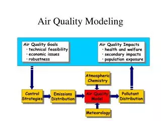
Meteorological Model Emission Model Chemical Model Temporal and spatial emission rates Topography Chemical Transformation Pollutant Transport Equilibrium between Particles and gases Vertical Mixing Source Dispersion Model Receptor Model Types of AQ Models
Emission Model • Estimates temporal and spatial emission rates based on activity level, emission rate per unit of activity and meteorology • Meteorological Model • Describes transport, dispersion, vertical mixing and moisture in time and space • Chemical Model • Describes transformation of directly emitted particles and gases to secondary particles and gases; also estimates the equilibrium between gas and particles for volatile species
Source Dispersion Model • Uses the outputs from the previous models to estimate concentrations measured at receptors; includes mathematical simulations of transport, dispersion, vertical mixing, deposition and chemical models to represent transformation. • Receptor Model • Infers contributions from different primary source emissions or precursors from multivariate measurements taken at one ore more receptor sites.
Classifications of AQ Models • Developed for a number of pollutant types and time periods • Short-term models – for a few hours to a few days; worst case episode conditions • Long-term models – to predict seasonal or annual average concentrations; health effects due to exposure • Classified by • Non-reactive models – pollutants such as SO2 and CO • Reactive models – pollutants such as O3, NO2, etc.
AQ Models • Classified by coordinate system used • Grid-based • Region divided into an array of cells • Used to determine compliance with NAAQS • Trajectory • Follow plume as it moves downwind • Classified by level of sophistication • Screening: simple estimation use preset, worst-case meteorological conditions to provide conservative estimates. • Refined: more detailed treatment of physical and chemical atmospheric processes; require more detailed and precise input data.
Fixed-Box Models • The city of interest is assumed to be rectangular. • The goal is to compute the air pollutant concentration in this city using the general material balance equation. Fig. 6.1 De Nevers
Fixed-Box Models Assumptions: Rectangular city. W and L are the dimensions, with one side parallel to the wind direction. Complete mixing of pollutants up to the mixing height H. No mixing above this height. The pollutant concentration is uniform in the whole volume of air over the city (concentrations at the upwind and downwind edges of the city are the same). The wind blows in the x direction with velocity u , which is constant and independent of time, location, & elevation.
… Assumptions The concentration of pollutant in the air entering the city is constant and is equal to b (for background concentration). The air pollutant emission rate of the city is Q (g/s). The emission rate per unit area is q = Q/A (g/s.m2). A is the area of the city (W x L). This emission rate is assumed constant. No destruction rate (pollutant is sufficiently long-lived)
Now, back to the general material balance eqn →Destruction rate = zero (from assumptions) →Accumulation rate = zero (since flows are independent of time and therefore steady state case since nothing is changing with time) → Q can be considered as a creation rate or as a flow into the box through its lower face. Let’s say a flow through lower face. Accumulation rate = (all flow rates in) – (all flow rates out) + (creation rate) – (destruction rate)
the general material balance eqn becomes: • The equation indicates that the upwind concentration is added to the concentrations produced by the city. • To find the worst case, you will need to know the wind speed, wind direction, mixing height, and upwind (background) concentration that corresponds to this worst case. 0 = (all flow rates in) – (all flow rates out) 0 = u W H b + q W L – u W H c Where c is the concentration in the entire city
Example 6.1 A city has the following description: W = 5 km, L = 15 km, u = 3 m/s, H = 1000 m. The upwind, or background, concentration of CO is b = 5 μg/m3. The emission rate per unit are is q = 4 x 10⁻⁶ g/s.m2. what is the concentration c of CO over the city? = 25 μg/m3
Comments on the simple fixed-box model • The fixed-box models does not distinguish between area sources and point sources. • Both sources are combined in the q value. We know that raising the release point of the pollutant will decrease the ground-level concentration. • So far, the fixed-box model predicted concentrations for only one specific meteorological condition. We know that meteorological conditions vary over the year.
Modifications to improve the fixed-box model 1) Hanna (1971) suggested a modification that allows one to divide the city into subareas and apply a different value of q to each. (since variation of q from place to place can be obtained; q is low in suburbs and much higher in industrial areas). 2) Changes in meteorological conditions can be taken into account by a. determine the frequency distribution of various values of wind direction, u, and of H b. Compute the concentration for each value using the fixed-box model
…Modifications to improve the fixed-box model c. Multiply the concentrations obtained in step b by the frequency and sum to find the annual average
Example 6.2 For the city in example 6.1, the meteorological conditions described (u = 3 m/s, H = 1000 m) occur 40 percent of the time. For the remaining 60 percent, the wind blows at right angles to the direction shown in Fig. 6.1 at velocity 6 m/s and the same mixing height. What is the annual average concentration of carbon monoxide in this city? First we need to compute the concentration resulting from each meteorological condition and then compute the weighted average. For u = 3 m/s and H = 1000 m → c = 25 μg/m3
…example 6.2 cont. Note that L is now 5km, not 15km For u = 6 m/s and H = 1000 m →
Gaussian Dispersion Models • Most widely used , Lakes Environnemental Software: http://www.weblakes.com • Plume spread and shape vary in response to meteorological conditions Fig. 6.3 De Nevers
X Z Q u Y H Fig 7.11
Model Assumptions • Gaussian dispersion modeling based on a number of assumptions including • Steady-state conditions (constant source emission strength) • Wind speed, direction and diffusion characteristics of the plume are constant. • Conservation of mass, i.e. no chemical transformations take place • Wind speeds are >1 m/sec. • Limited to predicting concentrations > 50 m downwind
The general equation to calculate the steady state concentration of an air contaminant in the ambient air resulting from a point source is given by: Where; c(x,y,z) = mean concentration of diffusing substance at a point (x,y,z) [kg/m3] x = downwind distance [m], y = crosswind distance [m], z = vertical distance above ground [m], Q = contaminant emission rate [mass/s], = lateral dispersion coefficient function [m], = vertical dispersion coefficient function [m], ῡ = mean wind velocity in downwind direction [m/s], H = effective stack height [m].
What are the A to F categories? • A to F are levels of atmospheric stability (table 6.1). • Explanation: • For a clear & hot summer morning with low wind speed, the sun heats the ground and the ground heats the air near it. Therefore air rises and mixes pollutants well. ►► Unstable atmosphere and large σy & σz values • On a cloudless winter night, ground cools by radiation to outer space and therefore cools the air near it. Hence, air forms an inversion layer. ►► Stable atmosphere and inhibiting the dispersion of pollutants and therefore small σy & σz values 2) Diffusion Models
Stability Classes • Table 3-1 Wark, Warner & Davis • Table 6-1 de Nevers
Dispersion Coefficients: Horizontal Fig 7.12
Dispersion Coefficients: Vertical Fig 7.13
Gaussian Dispersion Equation If the emission source is at ground level with no effective plume rise then Plume Rise • H is the sum of the physical stack height and plume rise.
Plume Rise This equation is only correct for the dimensions shown. Correction is needed for stability classes other than C: → For A and B classes: multiply the result by 1.1 or1.2 → For D, E, and F classes: multiply the result by 0.8 or 0.9 Δh = plum rise in m Vs = stack exit velocity in m/s D = stack diameter in m u = wind speed in m/s P = pressure in millibars Ts = stack gas temperature in K Ta = atmospheric temperate in K 2) Diffusion Models
Example 6.3 Q = 20 g/s of SO2 at Height H u = 3 m/s, At a distance of 1 km, σy = 30 m, σz = 20 m (given) Required: (at x = 1 km) SO2 concentration at the center line of the plume SO2 concentration at a point 60 m to the side of and 20 m below the centerline 30
8 2 6 7 9 1 13 14 11 3,4,5,12 10 Chemical Mass Balance Model • A receptor model for assessing source apportionment using ambient data and source profile data. • Available at EPA Support Center for Regulatory Air Models - http://www.epa.gov/scram001/tt23.htm PM10emissions from permitted sources in Alachua County (tons) (ACQ,2002) 2000 Values 1. GRU Deerhaven 144.2 2. Florida Rock cement plant 34.35 3. Florida Power UF cogen. plant 3.19 1997 Values 4. VA Medical Center incinerator 0.2 5. UF Vet. School incinerator 0.2 6. GRU Kelly 1.9 7. Bear Archery 9.5 8. VE Whitehurst asphalt plant 4.9 9. White Construction asphalt plant 0.7 10. Hipp Construction asphalt plant 0.3 11. Driltech equipment manufacturing 0.2 Receptor Sites 12. University of Florida 13. Gainesville Regional Airport 14. Gainesville Regional Utilities (MillHopper)
Principles Cij = Σ(aik×Skj) • Mass at a receptor site is a linear combination of the mass contributed from each of a number of individual sources; • Mass and chemical compositions of source emissions are conserved from the time of emission to the time the sample is taken. • Cij is the concentration of species ith in the sample jthmeasured at the receptor site: • aik is the mass fraction of the species in the emission from source kth, and • Skj is the total mass contribution from source kth in the jth sample at the receptor site.
Example • Total Pb concentration (ng/m3) measured at the site: a linear sum of contributions from independent source types such as motor vehicles, incinerators, smelters, etc PbT = Pbauto + Pb incin. + Pbsmelter +… • Next consider further the concentration of airborne lead contributed by a specific source. For example, from automobiles in ng/m3, Pbauto, is the product of two cofactors: the mass fraction (ng/mg) of lead in automotive particulate emissions, aPb, auto, and the total mass concentration (mg/m3) of automotive emission to the atmosphere, Sauto • Pbauto = aauto(ng/mg) × Sauto (mg/m3air)
Assumptions • Composition of source emissions is constant over period of time, • Chemicals do not react with each other, • All sources have been identified and have had their emission characterized, including linearly independent of each other, • The number of source category (j) is less than or equal to the number of chemical species (i) for a unique solution to these equations, and • The measurement uncertainties are random, uncorrelated, and normally distributed (EPA, 1990).