Download

1 / 49
530 likes | 894 Views
Computer Science at Oxford. Stephen Drape Access/Schools Liaison Officer. Four myths about Oxford. There’s little chance of getting in It’s expensive College choice is very important You have to be very bright. Myth 1: Little chance of getting in. False!

E N D
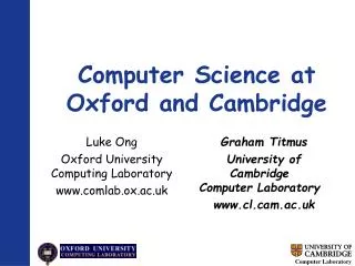
Computer Science at Oxford Stephen Drape Access/Schools Liaison Officer
Four myths about Oxford There’s little chance of getting in It’s expensive College choice is very important You have to be very bright
Myth 1: Little chance of getting in • False! • Statistically: you have a 20–40% chance Admissions data for 2007 entry:
Myth 2: It’s very expensive • False! • Most colleges provide cheap accommodation for three years. • College libraries and dining halls also help you save money. • Increasingly, bursaries help students from poorer backgrounds. • Most colleges and departments are very close to the city centre – low transport costs!
Myth 3: College Choice Matters • False! • If the college you choose is unable to offer you a place because of space constraints, they will pass your application on to a second, computer-allocated college. • Application loads are intelligently redistributed in this way. • Lectures are given centrally by the department as are many classes for courses in later years.
Myth 3: College Choice Matters • However… • Choose a college that you like as you have to live and work there for 3 or 4 years – visit if possible. • Look at accommodation & facilities offered. • Choose a college that has a tutor in your subject.
Myth 4: You have to be bright • True! • We find it takes special qualities to benefit from the kind of teaching we provide. • So we are looking for the very best in ability and motivation.
Our courses • Computer Science • Computer Science firmly based on Mathematics • Mathematics and Computer Science • Closer to a half/half split between CS and Maths • Courses can be for three or four years
Entrance Requirements • Essential: A-Level Mathematics • Recommended: Further Maths or a Science • Note it is not a requirement to have Further Maths for entry to Oxford • For Computer Science, Further Maths is perhaps more suitable than Computing or IT • Usual offer is AAA
Admissions Process • Fill in UCAS form • Choose a college or submit an “Open” Application • Interview Test • Based on common core A-Level • Taken before the interview • Interviews • Take place over a few days • Often have many interviews
Computer Science Year 1 Year 2 Year 3 Year 4 Mathematics Computing Project work
Mathematics & Computer Science Year 1 Year 2 Year 3 Year 4 Mathematics Computing Project work
Some of the different courses Functional Programming Design and Analysis of Algorithms Imperative Programming Digital Hardware Calculus Linear Algebra Logic and Proof
Useful Sources of Information • Admissions: • www.admissions.ox.ac.uk/ • Computing Laboratory: • www.comlab.ox.ac.uk/admissions/ • Mike Spivey’s info pages: • web2.comlab.ox.ac.uk/oucl/prospective/ugrad/csatox/ • College admissions tutors
What is Computer Science? It’s not about learning new programming languages. It is about understanding why programs work, and how to design them. If you know how programs work then you can use a variety of languages. It is the study of the Mathematics behind lots of different computing concepts.
Simple Design Methodology • Try a simple version first • Produce some test cases • Prove it correct • Consider efficiency (time taken and space needed) • Make improvements (called refinements)
Fibonacci Numbers The first 10 Fibonacci numbers (from 1) are: 1,1,2,3,5,8,13,21,34,55 The Fibonacci numbers occurs in nature, for example: plant structures, population numbers. Named after Leonardo of Pisa who was nicked named “Fibonacci”
The rule for Fibonacci The next number in the sequence is worked out by adding the previous two terms. 1,1,2,3,5,8,13,21,34,55 The next numbers are therefore 34 + 55 = 89 55 + 89 = 144
Using algebra To work out the nth Fibonacci number, which we’ll call fib(n), we have the rule: fib(n) = We also need base cases: fib(0) = 0 fib(1) = 1 This sequence is defined using previous terms of the sequence – it is an example of a recursive definition. fib(n – 1) + fib(n – 2)
Properties The sequence has a relationship with the Golden Ratio Fibonacci numbers have a variety of properties such as • fib(5n) is always a multiple of 5 • in fact, fib(a£b) is always a multiple of fib(a) and fib(b)
Writing a computer program Using a language called Haskell, we can write the following function: > fib(0) = 0 > fib(1) = 1 > fib(n) = fib(n-1) + fib(n-2) which looks very similar to our algebraic definition
Working out an example Suppose we want to find fib(5)
What’s happening? The program blindly follows the definition of fib, not remembering any of the other values. So, for (fib(3) + fib(2)) + fib(3) the calculation for fib(3) is worked out twice. The number of steps needed to work out fib(n) is proportional to n – it takes exponential time.
Refinements Why this program is so inefficient is because at each step we have two occurrences of fib (termed recursive calls). When working out the Fibonacci sequence, we should keep track of previous values of fib and make sure that we only have one occurrence of the function at each stage.
Writing the new definition We define > fibtwo(0) = (0,1) > fibtwo(n) = (b,a+b) > where (a,b) = fibtwo(n-1) > newfib(n) = fst(fibtwo(n)) The function fst means take the first number
Explanation The function fibtwo actually works out: fibtwo(n) = (fib(n), fib(n+1)) We have used a technique called tupling – this means that we keep extra results at each stage of a calculation. This version is much more efficient that the previous one (it is linear time).
Algorithm Design When designing algorithms, we have to consider a number of things: Our algorithm should be efficient – that is, where possible, it should not take too long or use too much memory. We should look at ways of improving existing algorithms. We may have to try a number of different approaches and techniques. We should make sure that our algorithms are correct.
Comments and Questions If there’s any comments or questions then please ask. There should be staff and students available to talk to Thank You
Finding the Highest Common Factor Example: Find the HCF of 308 and 1001. 1) Find the factors of both numbers: 308 – [1,2,4,7,11,14,22,28,44,77,154,308] 1001 – [1,7,11,13,77,91,143,1001] 2) Find those in common [1,7,11,77] 3) Find the highest Answer = 77
Creating an algorithm For our example, we had three steps: Find the factors Find those factors in common Find the highest factor in common These steps allow us to construct an algorithm.
Creating a program We are going to use a programming language called Haskell. Haskell is used throughout the course at Oxford. It is very powerful as it allows you write programs that look very similar to mathematical equations. You can easily prove properties about Haskell programs.
Step 1 We need produce a list of factors for a number n – call this list factor(n). A simple way is to check whether each number d between 1 and n is a factor of n. We do this by checking what the remainder is when we divide n by d. If the remainder is 0 then d is a factor of n. We are done when d=n. We create factor lists for both numbers.
Step 2 Now that we have our factor lists, which we will call f1 and f2, we create a list of common factors. We do this by looking at all the numbers in f1 to see if they are in f2. We there are no more numbers in f1 then we are done. Call this function: common(f1,f2).
Step 3 Now that we have a list of common factors we now check which number in our list is the biggest. We do this by going through the list remembering which is the biggest number that we have seen so far. Call this function: highest(list).
Function for Step 3 If list is empty then return 0, otherwise we check whether the first member of list is higher than the rest of list.
Putting the three steps together To calculate the hcf for two numbers a and b, we just follow the three steps in order. So, in Haskell, we can define Remember that when composing functions, we do the innermost operation first.
Problems with this method Although this method is fairly easy to explain, it is quite slow for large numbers. It also wastes quite a lot of space calculating the factors of both numbers when we only need one of them. Can we think of any ways to improve this method?
Possible improvements Remember factors occur in pairs so that we actually find two factors at the same time. If we find the factors in pairs then we only need to check up to n. We could combine common and highest to find the hcf more quickly (this kind of technique is called fusion). Could use prime numbers.
A Faster Algorithm This algorithm was apparently first given by the famous mathematician Euclid around 300 BC.
An example of this algorithm The algorithm works because any factor of a and b is also a factor of a – b hcf(308,1001) = hcf(308,693) = hcf(308,385) = hcf(308,77) = hcf(231,77) = hcf(154,77) = hcf(77,77) = 77
An even faster algorithm hcf(1001,308) 1001 = 3 × 308 + 77 = hcf(308,77) 308 = 4 × 77 = hcf(77,0) = 77
Computer Science Core CS 1(75%) Core Maths(25%) Year 1 Core CS 2(50%) CS Options(50%) Year 2 CS Options(25%) Advanced Options(50%) Project(25%) Year 3 Advanced Options(66%) Project(33%) Year 4(optional)
Mathematics & Computer Science Core 1(100%) Year 1 Core 2(58%) MathsOptions(17%) CS Options(25%) Year 2 MathsOptions(25-75%) CS Options(25-75%) Year 3 MathsOptions(25-75%) CS Options(25-75%) OptionalProject(33%) Year 4(optional)