v1.0 - 20050426

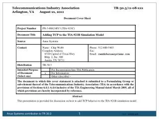
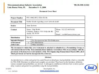
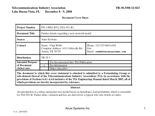
1. Telecommunications Industry Association TR-30.3/08-12-023 Lake Buena Vista, FL December 8 - 9, 2008 Anue Systems Inc v1.0 - 20050426

2. Load, Delay and Packet Loss TIA TR 30.3 meeting December 8-9, 2008 Orlando, FL

3. Goals • Improve TIA-921-A • Packet based Model • Correctly emulates impairment with different bit rate, packet size and packet intervals. Can handle mixed traffic. • Contrast with Time based model where the fixed packet size and packet interval must be specified. Cannot handle mixed traffic. • Variable bit rate user data (e.g. MPEG4 video) • Results depend on user packet sizes and when they arrive • Bidirectional network model (asymmetric) • Enforce bandwidth limits • Better correspondence between high latency and lost packets • Fewer “magic” numbers in the model • Fewer test cases TR 30.3 Meeting 12/8/2008

4. Disturbanceloadgenerator Output userpackets Input user packets LinkLatency + DisturbancePackets Goal: Understand this diagram. TR 30.3 Meeting 12/8/2008

5. Review of our previous work • Excellent proposal by Alan Clark to create a new model • The model takes into account traffic characteristics • Models typical TCP flow characteristics. • We discussed models used for G.8261 • Many similarities between TIA-921 and G.8261 • But enough differences to warrant a new effort • We discussed characteristics of disturbance loads • Burstiness definitions • Disturbance load probability density functions TR 30.3 Meeting 12/8/2008

6. Modeling strategies • Top down or bottom up • Many models are hybrids. • Top down models are constructed empirically • Observe behavior of the system under various conditions • Select parameter values that fits the observations • The parameters may or may not be physical properties of the system • Bottom up models are constructed analytically • Analyze how an idealized network component should behave • Parameters for these models are usually physical properties of the system • For example: buffer size in a router or switch • Test model components individually and compare the idealized results with actual measurements to verify. • If there’s a discrepancy, the idealized model must be revised TR 30.3 Meeting 12/8/2008

7. Modeling Strategies (cont.) • TIA-921 and TIA-921-A • A hybrid approach • These models are mainly top down models today • But have some bottom up characteristics • Some effects (such as serialization delay) derive from actual physical characteristics of the links • Other effects (such as core network behavior and link impulse probability) are empirically determined. • Goal for TIA-921-B is to build on previous work • Improved model should have more parts built bottom up. TR 30.3 Meeting 12/8/2008

8. The ultimate bottom-up model • We could build a discrete event simulation of every packet • But it is too computationally intensive. It requires that we simulate both packets of interest (user packets) and disturbance load packets. • A 24-hour simulation of a 10 hop network built out of GE switches and operating at 50% load with 1400 byte (avg) packets represents about 40 Billion packets. • That’s half a petabit. • If you watched HDTV for two years straight, without sleeping, it would use about that many bits. • Therefore it is not possible to simulate everything. We must make some approximations. TR 30.3 Meeting 12/8/2008

9. Strategy for simplification • Create a statistical model of the disturbance load traffic • Derive the delay and loss characteristics for different levels of disturbance loads. • Fully simulate all of the user packets • Use a statistical approximation of the disturbance load • Alan indicated he had information on characterizing typical TCP flows. • Last conference call, we talked about load PDFs • Statistical models of the disturbance packets • Result is a model that only needs to perform calculations when a user packet is received. • Significant increase in performance and accuracy. TR 30.3 Meeting 12/8/2008

10. Review: Burstiness • Define as an off and on process • Disturbance load generator is off or on • Definitions: • Nominal generator load is Lnom • While the generator is on, it creates a burst load Lburst • While the generator is off, it generates load of 0% • The time that the generator is on is Tburst (chosen randomly) • The time that the generator is off is Tgap • Choose a linear mapping for burst load • LBmin – Load during burst when Lnom= 0 • LBmax – Load during burst when Lnom= 100% TR 30.3 Meeting 12/8/2008

11. Review: Burstiness Equations TR 30.3 Meeting 12/8/2008

12. Review: Burstiness • LBmin= 50%, LBmax= 133% TR 30.3 Meeting 12/8/2008

13. Review: Composite Load PDF • Two CBR disturbance load generators • One bursty gamma disturbance load generator TR 30.3 Meeting 12/8/2008

14. Disturbanceloadgenerator + Idealized wire rate ethernet switch/router Input user packets Link Bit Rate R (bits/sec) Output userpackets Clock Crossing Fixed Latency Store & Forward Enqueue Delay Dequeue Delay LinkLatency Buffer SizeF(bits) DisturbancePackets TR 30.3 Meeting 12/8/2008

15. Idealized wire rate ethernet switch/router • Delay for idealized switch has several factors • Fixed latency • constant (approx 500ns) • Link latency • Time of flight for the signal (photons or electrons) • Store and Forward delay (serialization delay) • depends on user packet size (receive packet size/receive link rate) • Random • Clock crossing delay uncertainty (small, dozens of ns) • Enqueue and Dequeue latency (small, hundreds of ns) • Queuing delay • Load dependent • This is the hard part TR 30.3 Meeting 12/8/2008

16. Our example load PDF TR 30.3 Meeting 12/8/2008

17. ti-1 ti Delay and loss from disturbance load PDF • Assume that the queue starts out empty • We’ll revisit this assumption later, don’t worry • A user packet of size Si arrives at time ti • Define: • Step 1: • How much disturbance load arrived between ti-1 and ti? Si TR 30.3 Meeting 12/8/2008

18. Disturbance Load CDF • CDF is cumulative distribution function for PDF • Is piecewise continuous, monotonically increasing and invertible TR 30.3 Meeting 12/8/2008

19. Inverse CDF function (CDF-1) • The inverse CDF function can help • It is a mapping from uniform random numbers (easy to make) to random numbers of any distribution (hard to make) • This mapping can be pre-computed and saved in memory (very fast!) UniformRandomNumber TR 30.3 Meeting 12/8/2008

20. ti-1 ti Delay and loss from disturbance load PDF • A user packet of size Si arrives at time ti • Step 1: • How much disturbance load arrived between ti-1 and ti? • Generate by mapping a uniform random number through CDF-1 • Get a load percentage for ti: Li Si ? TR 30.3 Meeting 12/8/2008

21. Divide into three simpler sub-problems • Non-congested • Load is between 0 and LCONGEST (100%) • Congested • Load is between LCONGEST (100%) and LDROP • Overloaded • Load is more than LDROP • We’ll define LDROP in a moment TR 30.3 Meeting 12/8/2008

22. Three simpler sub-problems TR 30.3 Meeting 12/8/2008

23. Simplest sub-problem: Overload • Easiest sub-problem: the user packet gets dropped • This happens if the disturbance load percentage is so high that the queue is completely full when the user packet arrives. • Define LDROP as the load threshold above which a drop must occur. • If Li >= LDROP then the user packet is dropped • If F=16k bytes, R=100Mbit/second, and t=1ms, then LDROP=231% TR 30.3 Meeting 12/8/2008

24. Next simplest problem: non-congested • If 0 < Li < 100% then the queue will contain at most one disturbance load packet when the user packet arrives. The user packet is not dropped in this case. • Therefore it will be serviced immediately after any in-progress packet • Delay depends on the size of the disturbance packet (known), and when the user packet arrives relative to the disturbance packet (random). Assume arrival times are uncorrelated -> uniform RV. • Assume that the disturbance packets are E bits, which means that the maximum amount of time it has to wait (δ) is • So for this case, the delay is a uniform random value: [0.. δ] TR 30.3 Meeting 12/8/2008

25. Non-congested case: Example δ=110.4us TR 30.3 Meeting 12/8/2008

26. Non-Congested case: 50% TM2 • TM2 has 30%-64Byte, 10%-576Byte, 60%-1518Byte • So a 50% TM2 load is 15%,5%,30%. • This PDV histogram is often said to resemble a church or cathedral TR 30.3 Meeting 12/8/2008

27. See the characteristic “cathedral” shape of the PDV? Typical measured PDV Non-Congested case: Lab measurements TR 30.3 Meeting 12/8/2008

28. Congested case • Disturbance load 100% < Li < LDROP • Seems hard (but actually turns out to be simple) • We assumed that the buffer started out empty • (remember, we’ll fix this in a few more slides) • Conservation: • Bits added to queue during ti: Li * ti * R • Bits removed from queue during ti: ti * R • The difference is the buffer fullness (G) • And the delay is Gi/R TR 30.3 Meeting 12/8/2008

29. Adding memory • We assumed that the queue always started out empty • This essentially means that the time intervals (t) are independent • It is a reasonable approximation when the buffer size is much smaller than the number of bits serviced by the queue during t. • It’s usually a good approximation for high speed links • But not for low speed links like TIA-921 Access links • So, to fix that, save the queue state as a variable Gi • Need an equation to calculate Gi+1 • Change the threshold levels for LCONGEST and LDROP TR 30.3 Meeting 12/8/2008

30. Add memory • Adjust the thresholds LCONGEST and LDROP • Update equation for Gi (after calculation, Gi+1 is limited to be less than or equal to F) TR 30.3 Meeting 12/8/2008

31. Conclusion • Statistically modeling the disturbance load allows moreaccurate implementation of TIA-921-B • Supports • Variable bit rate user data (e.g. MPEG4 video) • Results depend on user packet sizes when they arrive • Bidirectional network model (assymetric) • Enforces bandwidth limits • Better correspondence between high latency and lost packets • Fewer “magic” numbers in the model TR 30.3 Meeting 12/8/2008

32. Next Steps • TBD TR 30.3 Meeting 12/8/2008