Download
1 / 41
410 likes | 497 Views
Learn to adjust for risk through varying discount rates, analyze sensitivity with graphs, conduct break-even NPV calculations, scenario analysis, and probability analysis to make informed project decisions.

E N D
LEARNING OBJECTIVES • Adjust for risk by varying the discount rate • Present a sensitivity graph and discuss • break-even NPV • Undertake scenario analysis • Make use of probability analysis to describe • the extent of risk facing a project and thus • make more enlightened choices • Discuss the limitations, explain the • appropriate use and make an accurate • interpretation of the results of the four risk • techniques described in this chapter
What is Risk? • Certainty • Risk and uncertainty • Objective probabilities • Subjective probabilities
ADJUSTING FOR RISK THROUGH THE DISCOUNT RATE Level of risk Risk-fr ee rate (%) Risk pr emium (%) Risk-adjusted rate (%) Low 9 +3 12 Medium 9 +6 15 High 9 +10 19 The pr oject cur r ently being consider ed has the following cash flows: T ime (years) 0 1 2 Cash flow (£) –100 55 70 If the pr oject is judged to be low risk: 55 70 NPV = –100 + + = +£4.91 2 (1 + 0.12) 1 + 0.12 Accept. If the pr oject is judged to be medium risk: 55 70 NPV = –100 + + = +£0.76 2 (1 + 0.15) 1 + 0.15 Accept. If the pr oject is judged to be high risk: 55 70 NPV = –100 + + = –£4.35 2 (1 + 0.19) 1 + 0.19 Reject.
Adjusting for risk • Drawbacks of the risk-adjusted discount rate method: • Risk classification is subjective • Difficulty in selecting risk premiums
SENSITIVITY ANALYSIS • Sensitivity analysis identifies the extent to which NPV changes as key variables are changed • A “what-if” analysis: • Acmart plc • new product line – Marts • likely demand for 1,000,000 a year • price of £1 • four-year life of product • initial investment £800,000 • Cash flow per unit £ • Sale price 1.00 • Costs • Labour 0.20 • Materials 0.40 • Relevant overhead 0.10 • 0.70 • Cash flow per unit 0.30 • Required rate of return = 15 per cent
NET PRESENT VALUE (1) Annual cash flow = 30p 1,000,000 = £300,000. Present value of annual cash flows = 300,000 annuity factor for 4 years @ 15% £ = 300,000 2.855 = 856,500Less initial investment –800,000 Net present value + 56,500
What if the price achieved is only 95p for • sales of 1m units (all other factors remaining • constant)? • Annual cash flow = 25p 1m = £250,000. • £ • 250,000 2.855 713,750 • Less initial investment 800,000 • Net present value –86,250 • What if the price rose by 1 per cent? • Annual cash flow = 31p 1m = £310,000. • £ • 310,000 2.855 885,050 • Less initial investment 800,000 • Net present value +85,050
What if the quantity demanded is 5 per cent • more than anticipated? • Annual cash flow = 30p 1.05m = £315,000. • £ • 315,000 2.855 899,325 • Less initial investment 800,000 • Net present value +99,325 • What if the quantity demanded is 10 per cent • less than expected? • Annual cash flow = 30p 900,000 = • £270,000. • £ • 270,000 2.855 770,850 • Less initial investment 800,000 • Net present value –29,150
What if the appropriate discount rate is 20 per • cent higher than originally assumed (that is, it • is 18 per cent rather than 15 per cent)? • 300,000annuityfactorfor 4 years@18% • £ • 300,000 2.6901 807,030 • Less initial investment 800,000 • +7,030 • What if the discount rate is 10 per cent lower • than assumed (that is, it becomes 13.5 per • cent)? • 300,000annuityfactorfor4 years @ 13.5%. • £ • 300,000 2.9441 883,230 • Less initial investment 800,000 • +83,230
100 50 NPV (£000) 0 Discount rate Sale –50 volume Sale price –100 –20 –15 –10 –5 0 5 10 15 20 25 % deviation of variable from expectation Sensitivity graph for Marts
Break-even NPV calculations • Advantages of using sensitivity analysis: • Information for decision making • To direct search • To make contingency plans • Drawbacks of sensitivity analysis: • No formal assignment of probabilities • Each variable is changed in isolation
SCENARIO ANALYSIS Observing NPV when numerous factors change Worst-case scenario Sales 900,000 units Price 90p Initial investment £850,000 Pr oject life 3 years Discount rate 17% Labour costs 22p Material costs 45p Over head 11p Cash flow per unit £ Sale price 0.90 Costs Labour 0.22 Material 0.45 Over head 0.11 0.78 Cash flow per unit 0.12 Annual cash flow = 0.12 900,000 = £108,000 £ Pr esent value of cash flows 108,000 2.2096 = 238,637 Less initial investment –850,000 Net pr esent value –611,363 Acmart plc: Project proposal for the production of Marts
SCENARIO ANALYSIS Best-case scenario Sales 1,200,000 units Price 120p Initial investment £770,000 Pr oject life 4 years Discount rate 14% Labour costs 19p Material costs 38p Over head 9p Cash flow per unit £ Sale price 1.20 Costs Labour 0.19 Material 0.38 Over head 0.09 0.66 Cash flow per unit 0.54 Annual cash flow = 0.54 1,200,000 = £648,000 £ Pr esent value of cash flows 648,000 2.9137 = 1,888,078 Less initial investment –770,000 Net pr esent value 1,118,078 Acmart plc: Project proposal for the production of Marts (continued)
PROBABILITY ANALYSIS Return Probability of return occurring Pr oject 1 16 1.0 Pr oject 2 20 1.0 Pr oject 3 –16 0.25 36 0.50 48 0.25 Pr oject 4 –8 0.25 16 0.50 24 0.25 Pr oject 5 –40 0.10 0 0.60 100 0.30 Pentagon plc: Use of probability analysis
EXPECTED RETURN The expected return is the mean or average outcome calculated by weighting each of the possible outcomes by the probability of occurrence and then summing the result. - x = x p + x p + ... x p 1 1 2 2 n n or i=n - x = ( x p ) i i i =1 - wher e x = the expected r etur n i = each of the possible outcomes (outcome 1 to n ) p = pr obability of outcome i occur ring n = the number of possible outcomes
Pentagon plc Expected returns Pr oject 1 16 1 16 Pr oject 2 20 1 20 Pr oject 3 –16 0.25 = –4 36 0.50 = 18 48 0.25 = 12 26 –2 Pr oject 4 –8 0.25 = 8 16 0.50 = 6 24 0.25 = 12 Pr oject 5 –40 0.1 = –4 0 0.6 = 0 100 0.3 = 30 26 Pentagon plc: expected returns
0.7 0.6 0.5 0.4 Probability 0.3 0.2 0.1 0 –100 –80 –60 –40 –16 0 20 36 48 80 100 £m Project 3 Project 5 Pentagon plc: Probability distribution for projects 3 and 5
2 STANDARD DEVIATION The standard deviation is a statistical measure of the dispersion around the expected value. The standard deviation is the square root of the variance - - - 2 2 2 2 V ariance of x = = ( x – x ) p + ( x – x ) p + ... ( x – x ) p x 1 1 2 2 n n i=n - 2 2 or = {( x – x ) p } x i i i =1 Standar d deviation i=n - 2 2 = or {( x – x ) p } x x i i i =1
Outcome Pr obability Expected Deviation Deviation Deviation (Return) r eturn squared squared times probability - - - - Pr oject xi pi x xi – x (xi – x )2 (xi – x )2pi 1 16 1.0 16 0 0 0 2 20 1.0 20 0 0 0 3 –16 0.25 26 –42 1,764 441 36 0.5 26 10 100 50 48 0.25 26 22 484 121 V ariance = 612 Standar d deviation = 24.7 4 –8 0.25 12 –20 400 100 16 0.5 12 4 16 8 24 0.25 12 12 144 36 V ariance = 144 Standar d deviation = 12 5 –40 0.1 26 –66 4,356 436 0 0.6 26 –26 676 406 100 0.3 26 74 5,476 1,643 V ariance = 2,485 Standar d deviation = 49.8 Pentagon plc: Calculating the standard deviations for the five projects
x Expected r etur n x Standar d deviation Pr oject 1 16 0 Pr oject 2 20 0 Pr oject 3 26 24.7 Pr oject 4 12 12 Pr oject 5 26 49.8 Pentagon plc: Expected return and standard deviation
RISK AND UTILITY Diminishing marginal utility Investment A Investment B Return Pr obability Retur n Probability Poor economic conditions 2,000 0.5 0 0.5 Good economic conditions 6,000 0.5 8,000 0.5 Expected r etur n 4,000 4,000 • Returns and utility • Risk averter • Risk lover
MEAN-VARIANCE RULE Project X will be preferred to Project Y if at least one of the following conditions apply: 1 The expected return of X is at least equal to the expected return of Y, and the variance is less than that of Y. 2 The expected return of X exceeds that of Y and the variance is equal to or less than that of Y.
30 Project 3 25 Project 5 Project 2 20 Project 1 Expected return 15 Project 4 10 5 0 0 12 24.7 49.8 Standard deviation Pentagon plc: Expected return and standard deviations
EXPECTED NET PRESENT VALUES AND STANDARD DEVIATION i=n NPV = ( NPV p ) i i i =1 wher e NPV = expected net pr esent value NPV = the NPV if outcome i occurs i p = pr obability of outcome i occur ring i n = number of possible outcomes The standar d deviation of the net pr esent value is i=n 2 = {( NPV – NPV ) p } i i NPV i =1
Cash flow at end of Y ear 1 HORIZON PLC Purchase price, t0 £500,000 Refurbishment, t0 £200,000 £700,000 The Year 1 cash flows are as follows: Pr obability Good customer r esponse 0.6 100,000 Poor customer r esponse 0.4 10,000
HORIZON PLC Conditional probabilities for the second year If the first year elicits a good response then: Probability Cash flow at end of Year 2 1 Sales increase in second year 0.1 £2m or 2 Sales are constant 0.7 £1.6m or 3 Sales decrease 0.2 £0.8m If the first year elicits a poor response then: Probability Cash flow at end of Year 2 1 Sales fall further 0.5 £0.7m or 2 Sales rise slightly 0.5 £1.2m Note: All figures include net trading income plus sale of pub.
Cash Probability Cash Conditional Cash Joint Outcome flow at p flow at probability flow at probability i T ime 0 T ime 1 T ime 2 (£000s) (£000s) (£000s) 2,000 0.6 0.1 = 0.06 a 0.1 0.7 1,600 0.6 b 100 0.6 0.2 800 0.6 c –700 700 0.4 0.5 = 0.20 d 0.5 0.4 10 0.5 1,200 0.4 0.5 = 0.20 e 1.00 An event tree showing the probabilities of the possible returns for Horizon plc
Net pr esent values NPV Pr obability (£000 s) 1,600 (1.1)2 Expected net pr esent value Outcome 2,000 100 a –700 + + = 1044 1,044 0.06 = 63 1.1 (1.1)2 100 713 0.42 b –700 + + = 713 = 300 1.1 800 100 c –700 + + = 52 = 6 52 0.12 (1.1)2 1.1 700 10 d –700 + + = –112 = –22 –112 0.20 1.1 (1.1)2 10 1,200 301 0.20 e –700 + + = 301 = 60 1.1 (1.1)2 407 or £407,000 Expected net present value, Horizon plc
i p 2 ) NPV ed times 367 2,247 obability Deviation 24,346 39,327 15,123 53,872 134,915 £367,000 – i squar pr NPV = = ( or 2 Variance ) 134,915 – NPV 93,636 11,236 405,769 126,025 269,361 Deviation squared i NPV ( d deviation = – NPV Deviation 637 306 –355 –519 –106 i Standar NPV Exhibit 6.17 Standard deviation for Horizon plc 407 407 407 407 407 NPV Expected NPV i 0.12 0.42 0.20 0.20 Probability p 0.06 52 713 301 1,044 –112 i £000s Outcome NPV b d a c e
Independent Probabilities The initial cash out flow = £150,000
THE RISK OF INSOLVENCY Probability 68.26 per cent 95.44 per cent 99.74 per cent X –3 –2 –1 +1 +2 +3 Standard deviations Exhibit 6.21 The normal curve
Probability 34.13 per cent Probability 68.26 per cent 95.44 per cent 99.74 per cent X –3 –2 –1 +1 +2 +3 Standard deviations Exhibit 6.22 Probability of outcome being between expected return and one standard deviation from expected return
THE Z STATISTIC Z = where: Z is the number of standard deviations from the mean X is the outcome that you are concerned about is the mean of the possible outcomes is the standard deviation of the outcome distribution X –
V alue of the Pr obability that X lies Z statistic within Z standar d deviations above (or below) the expected value (%) 0.0 0.00 0.2 7.93 0.4 15.54 0.6 22.57 0.8 28.81 1.0 34.13 1.2 38.49 1.4 41.92 1.6 44.52 1.8 46.41 2.0 47.72 2.2 48.61 2.4 49.18 2.6 49.53 2.8 49.74 3.0 49.87 Exhibit 6.23 The standard normal distribution
Probability Probability 47.72 per cent X –3 –2 –1 +1 +2 +3 £–5m £+8m Outcome Exhibit 6.24 Probability of outcome between and 2 from Roulette plc Maximum loss = £5m Expected return = £8m Standard deviation = £6.5m
PROBLEMS OF USING PROBABILITY ANALYSIS • Too much faith can be placed in quantified • subjective probabilities • Too complicated for all managers to understand • Projects may be viewed in isolation