Download

1 / 25
250 likes | 376 Views
A comparison of CRM simulations of trade wind cumulus with aircraft observations taken during RICO. Steve Abel and Ben Shipway 21 st Sept 2006 GCSS Workshop, New York. Overview.

E N D
A comparison of CRM simulations of trade wind cumulus with aircraft observations taken during RICO Steve Abel and Ben Shipway 21st Sept 2006 GCSS Workshop, New York
Overview • Currently most convection schemes distinguish between only two physical modes of cumulus convection – shallow and deep. • Work is under way at the Met Office to incorporate a third mode into the Unified Model (NWP and Climate) - warm rain cumulus (congestus) • This has involved running a number of idealized experiments using the Met Office Large Eddy Model (LEM) to simulate a range of congestus scenarios. • Observations from RICO allow us to test how well the LEM simulations were doing. • Compare the properties of updraft cores in the LEM with aircraft data. • Find that there are deficiencies in the original set up in the LEM – the model cannot reproduce the observed amounts of cloud and rain water contents. • Test the LEM response to changes in the model variables. • Can we make the LEM perform better? Abel and Shipway, submitted to QJ
Environmental Profiles (19th Jan 2005) Grey area shows the approximate range of the S-Pol radar. Filled circles show the launch location of the C-130 dropsondes. Open circle on south-east tip of Barbuda is the radiosonde launch site. Black line shows the mean of observations made on the 19th January 2005. Included are twelve dropsondes from the C-130 aircraft (12:18:58 – 19:40:01 UTC) and three radiosondes released from Barbuda (04:56:27 – 18:08:03 UTC).
Radar Imagery (19th January 2005) • Towering Cu in SPol radar domain for much of the day with extensive rain shafts. Later on these organised lines moved to SW and were replaced with a shallower field of trade wind Cu with less precipitation. • Observations used to initiate the LEM taken from ~ 5:00 – 20:00 UTC • Whilst the idealised LEM simulations are not designed to replicate the observed variability, the fairly heavy precipitation on this day will be a good test of the warm rain process in the model. S-Pol radar quick look images for selected times on the 19/01/2005. The images are centred on the island of Barbuda where the S-Pol radar was based.
Model forcing The model forcing (large scale subsidence plus temperature and moisture tendencies) was set up to induce quasi-equilibrium simulations with a profile similar to the observations following the methodology of Grant and Lock (2004), QJ.
Black line shows the mean of observations made on the 19th January 2005. Included are twelve dropsondes from the C-130 aircraft (12:18:58 – 19:40:01 UTC) and three radiosondes released from Barbuda (04:56:27 – 18:08:03 UTC). The red line is the equilibrium profile of the LEM. Environmental Profiles • Fairly moist layer below the trade wind inversion at 650 – 600 hPa (~ 4 km altitude) and above the sub-cloud boundary layer at ~ 950 hPa. • Above this the air is much drier and stable, indicative of high level subsidence. • Trade wind layer is slightly moister and the inversion stronger in the LEM than in the observations. • Horizontal wind also based on measured profiles.
Model setup: Domain size • 40 x 40 km (25.6 x 25.6 km) domain. Model top at 10 km. • 250 m (100 m) horizontal resolution. • High resolution run more similar to 1 Hz aircraft data (air speed ~ 100 ms-1) • 100 layers on a stretched grid in the vertical. • 40 m in the boundary layer • increasing to 100 m in the mid-troposphere up to 7 km • further degraded to 200 m towards top of domain
Time Series • Statistics taken from 18 hours onwards • Cloud top ~ 3.5 – 4 km • Cloud base ~ 350 – 400 m • Discrete peaks in rain rate indicate that only a few convective events are responsible for the majority of rainfall across domain at any one time
Typical Cloud Field Simulated by LEM Visualization of 3D fields
View from above 40 km GOES-12 ch1 image at 13:45 UTC on 19/01/05 • Similar features are evident in the satellite imagery and the LEM simulations. ~ 100 km Barbuda
Single moment rain Rain mixing ratio prognosed Rain droplet size distribution cannot be accurately represented Errors in sedimentation (size separation) and accumulation processes Poor representation of the warm rain processes Double moment rain Rain mixing ratio and number concentration prognosed Rain droplet size distribution more accurately represented Sedimentation (size separation) and accumulation processes more realistic Better representation of the warm rain processes Test sensitivity of LEM to changes in the model variables • Rain microphysics formulation 1) Single moment (1-M) vs Double moment (2-M) scheme
Test sensitivity of LEM to changes in the model variables 2) Rain Droplet fall speed • Fall flux of rain determined by mass weighted terminal velocity integrated over all droplet sizes. • The rain droplet fall speed is constrained to take the form of a modified gamma distribution. • However, the default fall speed (red line) can be improved upon. • We test out 2 other approximations for the fall speed (Smith – blue line & Uplinger – cyan line) Approximations to the droplet fall speed. Black line comes from theoretical results of Beard (1976).
Test sensitivity of LEM to changes in the model variables 3) Auto-conversion • The auto-conversion of cloud droplets to rain droplets is dependent upon the mixing ratio of cloud LWC, and the number concentration of cloud droplets, nl (i.e. dependent on mean drop diameter). • nl is set to a constant 2.4x10⁸ m-3 by default - RICO observations suggest a value of 5x10⁷ m-3 may be more appropriate. c.f. 4.5x10⁷ m-3 for RICO GCSS case • Reducing this value should enable cloud water to be more readily converted to rain. • Forcing strength Double the forcing in the model • Model Resolution Increase the horizontal resolution
Simulation features: Area averaged properties * * Radar data courtesy of Louise Nuijens and Bjorn Stevens
Comparing LEM simulations with aircraft observations In situ aircraft measurements of cloud updraft cores Observations of the atmospheric profile used to initialize LEM Generate simulated flight paths Compare the properties of cloud updraft cores simulated by the LEM with the in situ aircraft measurements Change LEM microphysics, resolution, forcing etc
0.05 gm-3 1 ms-1 Definition of a cloud updraft core • Updraft Core Penetration • Vertical velocity ≥ 1ms-1 and cloud LWC ≥ 0.05 gm-3 for at least 500 m along the flight track. Similar definition to previous aircraft studies of updrafts in stronger convective systems over the Tropical Pacific and Amazon regions (Anderson et al. 2005)
1-M versus 2-M • Better representation of rain droplet size distribution in 2-M scheme leads to a • decrease in cloud LWC • increase in rain LWC • decrease in number of • updrafts
Sensitivity to rain fall speed • Vertical distribution of rain LWC sensitive to droplet fall speed • Smith – Large droplets (2-4 mm) fall out too quickly low rain LWC, Reduced collection efficiency high cloud LWC • Uplinger – more realistic representation of fall speed c.f. Smith or default
Sensitivity to cloud droplet number conc. • Reducing nlin the auto-conversion scheme allows cloud water to be converted to rain more easily • Better agreement with observations in both cloud and rain LWC profiles
Sensitivity to equilibrium forcing • Doubling forcing leads to • ~ x 2 number updrafts • little change to mean profiles • larger surface rain rate due to more convective cells • Consistent with previous studies of deep convection e.g Schutts and Gray (1999), QJ
Sensitivity to horizontal resolution • Horizontal res 250 100 m • Decrease in updraft size • Increase in vertical velocity below 1.5 km • Shifts peak in rain LWC to higher up in cloud layer (large rain drops transported higher in updrafts)
Sampling Biases • Aircraft tends to sample larger updrafts • Result of aircraft aiming for larger visible clouds or that the LEM in not simulating the distribution of cloud size correctly. Further comparisons with satellite data would be required • Correlation between updraft size and both vertical velocity and rain LWC • No significant change in cloud LWC with updraft size
Summary • Default set-up of the LEM was not able to replicate the observed profiles of cloud and rain LWC in updrafts. • Increasing the forcing results in a greater number of updrafts in the model albeit with similar properties. • Vertical distribution of cloud and rain LWC is sensitive to droplet fall velocity. • High resolution run has a peak in rain LWC higher in updraft due to increased vertical velocity < 1.5 km • Lowering the concentration of cloud droplets required to initiate the auto-conversion scheme brings the model into better agreement with the observations of both cloud and rain water contents. • LEM is also able to produce surface rain rates that are in accordance with radar observations.