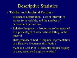
Data observation and Descriptive Statistics
Data observation and Descriptive Statistics. Organizing Data. Frequency distribution Table that contains all the scores along with the frequency (or number of times) the score occurs. Relative frequency: proportion of the total observations included in each score. . Frequency distribution.

Data observation and Descriptive Statistics
E N D
Presentation Transcript
Organizing Data • Frequency distribution • Table that contains all the scores along with the frequency (or number of times) the score occurs. • Relative frequency: proportion of the total observations included in each score.
Organizing data • Class interval frequency distribution • Scores are grouped into intervals and presented along with frequency of scores in each interval. • Appears more organized, but does not show the exact scores within the interval. • To calculate the range or width of the interval: • (Highest score – lowest score) / # of intervals • Ex: 120 – 0 / 5 = 24
Graphs • Bar graphs • Data that are collected on a nominal scale. • Qualitative variables or categorical variables. • Each bar represents a separate (discrete) category, and therefore, do not touch. • The bars on the x-axis can be placed in any order.
Graphs • Histograms • To illustrate quantitative variables • Scores represent changes in quantity. • Bars touch each other and represent a variable with increasing values. • The values of the variable being measured have a specific order and cannot be changed.
Frequency polygon • Line graph for quantitative variables • Represents continuous data: (time, age, weight)
Frequency Polygon AGE 22.06 24.05 25.04 25.04 25.07 25.07 26.03 26.11 27.03 27.11 29.03 29.05 29.05 34 37.1 53
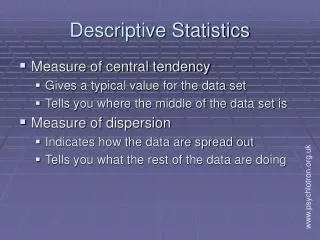
Descriptive Statistics • Numerical measures that describe: • Central tendency of distribution • Width of distribution • Shape of distribution
Central tendency • Describe the “middleness” of a data set • Mean • Median • Mode
_ X = ∑ X _____ n Mean • Arithmetic average • Used for interval and ratio data • Formula for population mean ( µ pronounced “mu”) µ = ∑ X _____ N • Formulas for sample mean
Mean • Not a good indicator of central tendency if distribution has extreme scores (high or low). • High scores pull the mean higher • Low scores pull the mean lower
Median • Middle score of a distribution once the scores are arranged in increasing or decreasing order. • Used when the mean might not be a good indicator of central tendency. • Used with ratio, interval and ordinal data.
Mode • The score that occurs in the distribution with the greatest frequency. • Mode = 0; no mode • Mode = 1; unimodal • Mode = 2; bimodal distribution • Mode = 3; trimodal distribution
Measures of Variability • Range • From the lowest to the highest score • Variance • Average square deviation from the mean • Standard deviation • Variation from the sample mean • Square root of the variance
Measures of Variability • Indicate the degree to which the scores are clustered or spread out in a distribution. • Ex: Two distributions of teacher to student ratio. Which college has more variation?
Range • The difference between the highest and lowest scores. • Provides limited information about variation. • Influenced by high and low scores. • Does not inform about variations of scores not at the extremes. • Examples: • Range = X(highest) – X (lowest) • College A: range = 41- 4 = 37 • College B: range = 22-16 = 6
Variance • Limitations of range require a more precise way to measure variability. • Deviation: The degree to which the scores in a distribution vary from the mean. • Typical measure of variability: standard deviation (SD) • Variance The first step in calculating standard deviation
Variance • X = Number of therapy sessions each student attended. • M = 4.2 “Deviation” Sum of deviations = 0
Variance • In order to eliminate negative signs, we square the deviations. • Sum the deviations = sum of squares or SS
Variance • Take the average of the SS • Ex: SS = 48.80 • SD2 = Σ(X-M)2 N • That is the average of the squared deviations from the mean • SD2 = 9.76
Standard Deviation • Standard deviation • Typical amount that the scores vary or deviate from the sample mean • SD = Σ(X-M)2 N • That is, the square root of the variance • Since we take the square root, this value is now more representative of the distribution of the scores. ____ √
Standard Deviation • X = 1, 2, 4, 4, 10 • M = 4.2 • SD = 3.12 (standard deviation) • SD2 = 9.76 (variance) • Always ask yourself: do these data (mean and SD) make sense based on the raw scores?
____ √ σ =∑( X - µ ) ² _________ N Population Standard Deviation • The average amount that the scores in a distribution vary from the mean. • Population standard deviation: (σpronounced “sigma”)
σ = ∑( X - µ ) ² _________ N Sample Standard Deviation • Sample is a subset of the population. • Use sample SD to estimate population SD. • Because samples are smaller than populations, there may be less variability in a sample. • To correct for this, we divide the sample by N – 1 • Increases the standard deviation of the sample. • Provides a better estimate of population standard deviation. √ √ s = ∑( X - X ) ² _________ N - 1 Unbiased Sample estimator standard deviation Population standard deviation
Types of Distributions • Refers to the shape of the distribution. • 3 types: • Normal distribution • Positively skewed distribution • Negatively skewed distribution
Normal Distribution • Normal distributions: Specific frequency distribution • Bell shaped • Symmetrical • Unimodal • Most distributions of variables found in nature (when samples are large) are normal distributions.
Normal Distribution • Mean, media and mode are equal and located in the center.
Skewed distributions • When our data are not symmetrical • Positively skewed distribution • Negatively skewed distribution Memory hint: skew is where the tail is; also the tail looks like a skewer and it points to the skew (either positive or negative direction)
Kurtosis • Kurtosis - how flat or peaked a distribution is. • Tall and skinny versus short and wide • Mesokurtic: normal • Leptokurtic: tall and thin • Platykurtic: short and fat (squatty like a platypus!)
Kurtosis leptokurtic platykurtic mesokurtic
Skewness, Number of Modes, and Kurtosis in Distribution of Housing Prices
z - Scores • In which country (US vs. England) is Homer Simpson considered overweight? • How can we make this comparison? • Need to convert weight in pounds and kilograms to a standardized scale. • Z- scores: allow for scores from different distributions to be compared under standardized conditions. • The need for standardization • Putting two different variables on the same scale • z-score: Transforming raw scores into standardized scores z = (X - µ) σ • Tell us the number of standard deviations a score is from the mean.
z- Scores • Class 1: M = $46.53 SD = $41.87 X = $54.76 • Class 2: M = $53.67 SD = $18.23 X = $89.07 • In which class did I have more money in comparison to the distribution of the other students? Sample z-score: z = (X - M) s • When we convert raw scores from different distributions to z-scores, these scores become part of the same z distribution and we can compare scores from different distributions.
z Distribution • Characteristics: (regardless of the original distributions) • z score at the mean equals 0 • Standard deviation equals 1
z distribution of exam scores M = 70 s = 10
Standard normal distribution • If a z-distribution is normal, then we refer to it as a standard normal distribution. • Provides information about the proportion of scores that are higher or lower than any other score in the distribution.
Standard Normal Curve Table • Standard normal curve table (Appendix A) • Statisticians provided the proportion of scores that fall between any two z-scores. • What is the percentile rank of a z score of 1? • Percentile rank = proportion of scores at or below a given raw score. • Ex: SAT score = 1350 M = 1120 s = 340 • 75th percentile
Percentile Rank The percentage of scores that your score is higher than. • 89th percentile rank for height • You are taller than 89% of the students in the class. (you are tall!) • Homer Simpson: 4th percentile rank for intelligence. he is smarter than 4% of the population (or 96% of the population is smarter than Homer). • GRE score: 88th percentile rank • Reading scores of grammar school: 18th percentile rank
Review • Data organization • Frequency distribution, bar graph, histogram and frequency polygon. • Descriptive statistics • Central tendency = middleness of a distribution • Mean, median and mode • Measures of variation = the spread of a distribution • Range, standard deviation • Distributions can be normal or skewed (positively or negatively). • Z- scores • Method of transforming raw scores into standard scores for comparisons. • Normal distribution: mean z-score = 0 and standard deviation = 1 • Normal curve table: shows the proportions of scores below the curve for a given z-score.


