Download
1 / 5
50 likes | 193 Views
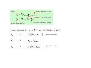
Optimal prediction of x. Optimal prediction of y. EKF - Equations. x(k)=[x,y,th]. T=sample time interval. state. input.

E N D
Optimal prediction of x Optimal prediction of y
x(k)=[x,y,th] T=sample time interval
state input To propagate the error covariance matrix associated with the state matrix to the next stage, the error incurred is assumed to be small so that first order Taylor’s expansion in the form of Jacobian matrix does not introduce significant higher order errors. Given the error covariance matrix of Sk-1 and the input vector u, and given the intuition that the error in stage k-1 is not correlated with the error introduced by the input, the covariance matrix of the next stage, k, can be evaluated as follows, where the major problem with this treatment is that there is no physical basis in assuming that the translation error is uncorrelated with the rotation error http://www.ecse.monash.edu.au/centres/IRRC/LKPubs/ODOMTECH.PDF