Download
1 / 13
140 likes | 384 Views
The Taylor Series. 1 ’ st Taylor Series. The Principle of derivation Eule’s/modified Eule’s. Mechanical System. K. Mass m. m. b. From Newton’s law. Spring Constant k=1 N/m m=1 kg , Viscous Coefficient b=0.3 N/m/sec. Simulation (I). Let % The Mechanical System

E N D
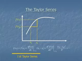
The Taylor Series 1’st Taylor Series
Mechanical System K Mass m m b From Newton’s law Spring Constant k=1 N/m m=1 kg , Viscous Coefficient b=0.3 N/m/sec
Simulation (I) • Let % The Mechanical System clear; x1=2;x2=0;dt=0.01; for k=1:2000 t(k)=k*dt; x1=x2*dt+x1; x2=(-0.3*x2-x1)*dt+x2; pos(k)=x1;vel(k)=x2; end plot(t,pos,’r’);
Simulation (II) Plot(t,pos,’r’); hold; plot(t,vel,’b’); subplot(2,2,1); plot(t,pos,’r’); subplot(2,2,2); plot(t,vel,’b’); subplot(2,2,3); plot(pos,vel,’g’);
ODE45 to solve differential equation • Initial Value Problem (IVP) • Example: Van der Pol Equation • ODE Program –ode45 Before a D.E can be solved, they must be coded in a function M-file ydot=odefile(t,y) format 指令 – format long/format short
Program of Vdpol function ydot=vdpol(t,y) mu=2; ydot=[y(2);mu*(1-y(1)^2)*y(2)-y(1)]; tspan=[0 20]; y0=[2 0]; [t,y]=ode45(@vdpol,tspan,y0); % [t,y]=ode45(‘vdpol’,tspan,y0);plot(t,y(:,1),t,y(:,2),’r-’); xlabel(‘Time’) title(‘Van der Pol Solution’)
HW1 Force Term – Step Input f(0~2 s) Mass m Friction Force f=1N , m=1kg , b=0.4N/m/sec Plot the response of position and velocity
Wheeled Mobile Robot • Consider the following kinematic Model of Mobile Robot,
Homework 1: Deadline up to f(0~0.5s) Mass m Length=8m Friction m=1kg , b=0.5N/m/sec (1) 試以模擬結果推論, 當物體剛好移動 8m 需要多少 Nt 力量 (2) 當物體速度為最大時, 位移為何? 歷時多久? (3) 當物體移動了 2m, 4m, 6m 速度分別為何? 分別歷時為何?
HW2 : Electric Network : L-R-C Series Circuit L=2 R=1.5 C=0.3 i (1) 繪出電容電壓與流過電容之電流之相位平面圖 (2) 時間為 1, 3, 5, 7 (s), 電容電壓與流过電容兩端電流分別為何? (3) 模擬結果, 電容電壓會振盪嗎? 改變 C 的大小, 能否使得電容 電壓在充電過程中不會振盪, 能夠寫出系統是否振盪的判斷準則?
HW3 : Pendulum System (c) 當擺槌速度為 0 時,時間為何? 請分別列出.
HW4 : Compare the accurate between Euler method, ODE45 and Runge-Kutta method • Using Engineering Mathematics method to calculate the solution • of the above differential equation by hand. (2) Compare the simulation results of three method, and sketch the output response (y) in the same figure. (3) Could you give a conclusions for the comparison of above approaches.