Download
1 / 15
150 likes | 295 Views
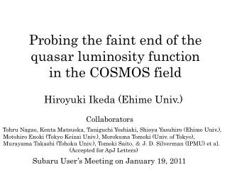
Probing the faint end of the quasar luminosity function in the COSMOS field. Hiroyuki Ikeda (Ehime Univ.). Collaborators. Tohru Nagao, Kenta Matsuoka, Taniguchi Yoshiaki, Shioya Yasuhiro (Ehime Univ.),

E N D
Probing the faint end of the quasar luminosity function in the COSMOS field Hiroyuki Ikeda (Ehime Univ.) Collaborators Tohru Nagao, Kenta Matsuoka, Taniguchi Yoshiaki, Shioya Yasuhiro (Ehime Univ.), Motohiro Enoki (Tokyo Keizai Univ.), Morokuma Tomoki (Univ. of Tokyo), Murayama Takashi (Tohoku Univ.), Tomoki Saito, & J. D. Silverman (IPMU) et al. (Accepted for ApJ Letters) Subaru User’s Meeting on January 19, 2011
Table of Contents ・Introduction ・Data and Sample Selection ・Completeness Estimation ・QSO Luminosity Function ・Summary
<Introduction> We have focused on the QSO Luminosity Function to study the evolution of SMBHs. QSO Luminosity Function z~ 0.5 - 3 z ~ 4 - 5 0.40<z<0.68 0.68<z<1.06 1.06<z<1.44 1.44<z<1.82 1.82<z<2.20 2.20<z<2.60 10-5 10-6 10-7 10-8 ●: 3.6 < z < 3.9 ▲: 3.9 < z < 4.4 ○: 4.4 < z< 5.0 Space Density (Mpc-3 mag-1) Fan et al. (2001) Croom et al. (2009) -20 -22 -24 -26 -28 Mg No Data
<Data and Sample Selection> • ・Survey Area:COSMOS Field (2deg2) • Data:COSMOS photometric catalog • Subaru/Suprime-Cam: Data of the g’, r’, i’, z’ filter • HST/ACS: Data of the F814W (i) • •Sample Selection • (1) • (2)Two-color diagram (g’−r’ vs. r’–i’) Point source on the HST image and 22 < i’ < 24. 31 candidates at z ~ 4
<Spectroscopic Follow-up (Subaru/FOCAS)> 8 objects show strong and broad Lyα and C iv emission lines!
<Photometric Completeness> We have estimated the completeness through detailed Monte Carlo simulations by QSO model spectra. Completeness is not 1 at i’<22. →Bright Objects that exist foreground →Individuality of QSOs →Photometric Error due to this 3 effects
< QSO Luminosity Function at z ~ 4> Our QLF at z ∼ 4 has a much shallower faint-end slope than that obtained by other recent surveys in the same redshift.
<Evolution of the QSO Space Density> Our result is consistent with the scenario of downsizing Evolution of AGN inferred by recent optical quasar surveys at lower redshifts.
<Summary> ・We have surveyed high redshift QSOs in the COSMOS field. ・We have discovered 8 low luminosity QSOs at z ~ 4. ・We have estimated the completeness through detailed Monte Carlo simulations by QSO model spectra. ・Our QLF at z ~ 4 has a much shallower faint-end slope than that obtained by other recent surveys in the same redshift. •Our result is consistent with the scenario of downsizing evolution of AGN inferred by recent optical quasar surveys at lower redshifts.
Two color diagram (g’r’i’) <Selection Criteria> :Color truck of the model QSO (1)g’-r’ > 1.0 (2)r’-i’<0.42(g’-r’)-0.22 (3)u-g’ > 2.0 ×:Point source(22<i’<24) r’-i’ z 〜 4.7 Area of the QSO candidate z〜 3.7 31 candidates at z ~ 4 g’-r’
QSO Model Spectra We have made QSO model spectra to determine our photometric completeness. <αν>=0.46、σαν=0.3 <EW(Lyα)>=90Å、σEW=20Å Flux Density (arbitrary units) 1000 5000 Wavelength(Å)
SDSS DR7 QSO colors and simulated QSO colors • SDSS DR7 QSO Model QSO (Bar = ±1σ)
<How to determine the completeness> ・We assume that i’-band magnitude equals 22. So, we can determine the other band magnitude. ・We insert model QSOs into the COSMOS images, using the IRAF mkobjects task in the artdata package. ・We extract the model QSOs by SExtractor. ・We count up these objects that satisfy our selection criteria, and we determine the completeness.
Two color diagram at z~ 4 十 ; QSO × ;Not QSO ; Color truck of the model QSO r’-i’ g’-r’