Download
1 / 57
570 likes | 830 Views
Lecture 7 Carry look ahead adders, Latches, Flip-flops, registers, multiplexors, decoders Digital Works intro PH 3 : Appendix B.6-9. Adders. Last time we developed a 32 bit ripple adder. It is not an efficient adder, although simple to understand, so how can we improve its performance.

E N D
Lecture 7Carry look ahead adders,Latches, Flip-flops, registers, multiplexors, decodersDigital Works introPH 3 : Appendix B.6-9 Chapter 1 — Computer Abstractions and Technology — 1
Adders • Last time we developed a 32 bit ripple adder. • It is not an efficient adder, although simple to understand, so how can we improve its performance. • We will try to see what can be done to speed it up. Chapter 1 — Computer Abstractions and Technology — 2
Problem: ripple carry adder is slow • Is a 32-bit ALU as fast as a 1-bit ALU? • Is there more than one way to do addition? • two extremes: ripple carry and sum-of-products Can you see the ripple? How could you get rid of it? c1 = b0c0 + a0c0 +a0b0 c1 = (b0 + a0)c0 +a0b0 c2 = b1c1 + a1c1 +a1b1 c2 = (b1 + a1)c1 +a1b1 c3 = b2c2 + a2c2 +a2b2 c3 = … c4 = b3c3 + a3c3 +a3b3 c4 = … — 3
Carry-lookahead adder • An approach in-between our two extremes • Motivation: • If we didn't know the value of carry-in, what could we do? • Let gi = ai bi , called generate, and , pi = ai + bi , called propagate. Now the equations can be written as below c1 = g0 + p0c0 c2 = g1 + p1c1 = g1 + p1(g0 + p0c0) c3 = g2 + p2c2 = g2 + p2(g1 + p1(g0 + p0c0)) c4 = g3 + p3c3 = ... So we see it is possible to generate however many carries we desire that are independent of all carries except c0. However it tends to become quite expensive in terms of numbers of gates. So what can we do? — 4
A four bit carry lookahead adder Chapter 1 — Computer Abstractions and Technology — 5
Cascade connection of 4-bit carry lookahead adders. Can’t build a 16 bit adder this way... (too big) Could use ripple carry of 4-bit CLA adders Better: use the CLA principle again! Chapter 1 — Computer Abstractions and Technology — 6
Memory Simple Flip-Flop Applications Chapter 1 — Computer Abstractions and Technology — 7
Basic bistable element. Chapter 1 — Computer Abstractions and Technology — 8
SR (set-reset) latch. (a) Logic diagrams. (b) Function table where Q+ denotes the output Q in response to the inputs. (c) Two logic symbols. Chapter 1 — Computer Abstractions and Technology — 9
An application of the SR latch. (a) Effects of contact bounce. (b) A switch debouncer. Chapter 1 — Computer Abstractions and Technology — 10
latch. (a) Logic diagrams. (b) Function table where Q+ denotes the output Q in response to the inputs. (c) Two logic symbols. Chapter 1 — Computer Abstractions and Technology — 11
Gated SR latch. (a) Logic diagram. (b) Function table where Q+ denotes the output Q in response to the inputs. (c) Two logic symbols (c) Chapter 1 — Computer Abstractions and Technology — 12
Gated D latch. (a) Logic diagram. (b) Function table where Q+ denotes the output Q in response to the inputs. (c) Two logic symbols. Chapter 1 — Computer Abstractions and Technology — 13
Timing diagram for an SR latch. Chapter 1 — Computer Abstractions and Technology — 14
Timing diagram for a gated D latch. Chapter 1 — Computer Abstractions and Technology — 15
Positive-edge-triggered D flip-flop. (a) Logic diagram. (b) Function table where Q+ denotes the output Q in response to the inputs. (c) Two logic symbols. Chapter 1 — Computer Abstractions and Technology — 16
Positive-edge-triggered D flip-flop • NAND gates 5 and 6 serve as an latch. Thus as long as S = R = 0, i.e. S’ = R’ = 1, the state of the latch cannot change; while whenever S or R is 1, i.e. S’ or R’ is 0, but not both the latch sets or resets. • Now if C = 0 the outputs of gates 2 and 3 are 1, regardless of D, so the latch does not change. • Now assume D = 0. then the output at gate 4 is 1 and at gate 1 is 0 since the outputs at gates 4 and 2 are 1. • When C goes from 0 to 1, the positive edge, all inputs to gate 3 become 1 so R’ = 0. But S’ remains 1 since the input from gate 1 is still 0 so Q = 0 and Q’ = 1. In addition the ouput 0 from gate 3 feeds back to gate 4 to keep the output there at 1 regardless of changes to D so long as C stays equal 1. Chapter 1 — Computer Abstractions and Technology — 17
Positive-edge-triggered flip-flop continued • Now suppose C = 0 and D = 1. As before the ouputs from gates 2 and 3 are 1 causing the S’R’ latch to hold its current state. However D = 1 causes the output of gate 4 to be 0 which causes the output of gate 1 to be 1. • Now when C changes to 1 both inputs to gate 2 become 1 so S’ = 0. R’ remains 1 since the input from gate 4 to gate 3 is 0. Now S’ = 0 and R’ = 1 causes Q = 1 and Q’ = 0. • The 0 output from gate 2 causes the outputs at gates 1 and 3 to remain at 1. Thus if D changes as long as C = 1, there will be no change in the S’R’ latch. Chapter 1 — Computer Abstractions and Technology — 18
Timing diagram for a positive-edge-triggered D flip-flop. Chapter 1 — Computer Abstractions and Technology — 19
General model of a sequential network. Chapter 1 — Computer Abstractions and Technology — 20
Logic Design Basics • Information encoded in binary • Low voltage = 0, High voltage = 1 • One wire per bit • Multi-bit data encoded on multi-wire buses • Combinational element • Operate on data • Output is a function of input • State (sequential) elements • Store information Chapter 1 — Computer Abstractions and Technology — 21
A Y B A A Mux I0 Y + Y Y I1 ALU B B S F Combinational Elements • AND-gate • Y = A & B • Adder • Y = A + B • Arithmetic/Logic Unit • Y = F(A, B) • Multiplexer • Y = S ? I1 : I0 Chapter 1 — Computer Abstractions and Technology — 22
Structure of a clocked synchronous sequential network. Chapter 1 — Computer Abstractions and Technology — 23
An m-bit register using D flip-flops Chapter 1 — Computer Abstractions and Technology — 24
Register File: Built using flip-flops Chapter 1 — Computer Abstractions and Technology — 25
Universal shift register. (a) Logic diagram. (b) Mode control. (c) Symbol. Chapter 1 — Computer Abstractions and Technology — 26
Do you understand? What is the “Mux”? — 27
Multiplexor • A multiplexor that chooses one of two words. Built by using 1 bit multiplexors and stringing them together as on the right. Chapter 1 — Computer Abstractions and Technology — 28
An n-to-2n-line decoder symbol. Chapter 1 — Computer Abstractions and Technology — 29
A 3-to-8-line decoder.(a) Logic diagram. (b) Truth table.(c) Symbol. Chapter 1 — Computer Abstractions and Technology — 30
Register File (Note: we still use the real clock to determine when to write) — 31
Simple Implementation • The functional units we need for each instruction — 32
Simple implementation continued. Functions needed for loads and stores Chapter 1 — Computer Abstractions and Technology — 33
Simple implementation continued. What happens to the instruction Chapter 1 — Computer Abstractions and Technology — 34
Introduction to Digital Works Chapter 1 — Computer Abstractions and Technology — 35
The Digital Works Window Chapter 1 — Computer Abstractions and Technology — 36
Creating and using Macros Converting the two-input multiplexer circuit into a black box Chapter 1 — Computer Abstractions and Technology — 37
Creating the black box • Left click on the arrow. • Right click on one of the macro tags. • Select Template Editor from the menu with a left click. • The Template Editor window appears. You can create a symbol for your circuit. There may already be a default black box and if there is you can use it if you like, or you can delete it and draw one that you like. Chapter 1 — Computer Abstractions and Technology — 38
Creating a symbol for the new circuit Chapter 1 — Computer Abstractions and Technology — 39
Procedure for building the macro • Once you have drawn an object or decided to use the default one you select the Pin Icon by left clicking. • You then place the cursor where you want it to be in the diagram and left click to insert it. • Next select it and right click and select associate with tag from the menu. • Next close the template editor. You will notice a 1 next to the selected macro tag. • Now select another macro tag, right click and select template editor and repeat the above procedure except for drawing the template. Do this for the remaining macro tags and then save the file. You do not use a separate name for the macro. Chapter 1 — Computer Abstractions and Technology — 40
Creating an interface point in the black box Chapter 1 — Computer Abstractions and Technology — 41
The completed black box representation Chapter 1 — Computer Abstractions and Technology — 42
The original circuit with the macro tags numbered Chapter 1 — Computer Abstractions and Technology — 43
Using a Macro Embedding a macro in a circuit Chapter 1 — Computer Abstractions and Technology — 44
Using a Macro continued • You can use the push button interactive tool to insert inputs to the macro and the LED tool to insert outputs to the macro. You then wire the interactive buttons and LEDs to the appropriate macro icons. You can then run and test it. • Suppose you want to build a circuit having more than one macro (which may or may not be the same) • Select the embed macro button and position the cursor to where you want it in the workspace and left click. Chapter 1 — Computer Abstractions and Technology — 45
Embedding two macros, wiring them together Chapter 1 — Computer Abstractions and Technology — 46
Editing a macro in a circuit Chapter 1 — Computer Abstractions and Technology — 47
Editing the expanded form of the macro Chapter 1 — Computer Abstractions and Technology — 48