Download
1 / 90
930 likes | 1.16k Views
Network Layer: Part II. Basic Routing Principles and Routing Algorithms Link State vs. Distance Vector Routing in the Internet Intra-AS vs. Inter-AS routing Intra-AS: RIP and OSPF Inter-AS: BGP and Policy Routing Broadcast and Multicast Routing (optional)

E N D
Network Layer: Part II • Basic Routing Principles and Routing Algorithms • Link State vs. Distance Vector • Routing in the Internet • Intra-AS vs. Inter-AS routing • Intra-AS: RIP and OSPF • Inter-AS: BGP and Policy Routing • Broadcast and Multicast Routing (optional) Readings: Textbook: Chapter 4, Sections 4.5-4.8 CSci4211: Network Layer: Part II
5 3 5 2 2 1 3 1 2 1 F D E B C A Routing & Forwarding:Logical View of a Router CSci4211: Network Layer: Part II
ICMP protocol • error reporting • router “signaling” Transport layer: TCP, UDP • IP protocol • addressing conventions • packet handling conventions • Routing protocols • path selection • RIP, OSPF, BGP routing table Data Link layer (Ethernet, WiFi, PPP, …) Physical Layer (SONET, …) IP Forwarding & IP/ICMP Protocol Network layer CSci4211: Network Layer: Part II
Routing: Issues • How are routing tables determined? • Who determines table entries? • What info used in determining table entries? • When do routing table entries change? • Where is routing info stored? • How to control routing table size? Answer these questions, we are done! CSci4211: Network Layer: Part II
Routing Paradigms • Hop-by-hop Routing • Each packet contains destination address • Each router chooses next-hop to destination • routing decision made at each (intermediate) hop! • packets to same destination may take different paths! • Example: IP’s default datagram routing • Source Routing • Sender selects the path to destination precisely • Routers forward packet to next-hop as specified • Problem: if specified path no longer valid due to link failure! • Example: • IP’s loose/strict source route option (you’ll see later) • virtual circuit setup phase in ATM (or MPLS) CSci4211: Network Layer: Part II
Routing Algorithms/Protocols Issues Need to Be Addressed: • Route selection may depend on different criteria • Performance: choose route with smallest delay • Policy: choose a route that doesn’t cross .gov network • Adapt to changes in network topology or condition • Self-healing: little or no human intervention • Scalability • Must be able to support large number of hosts, routers CSci4211: Network Layer: Part II
Centralized vs. Distributed Routing Algorithms Centralized: • A centralized route server collects routing information and network topology, makes route selection decisions, then distributes them to routers Distributed: • Routers cooperate using a distributed protocol • to create mutually consistent routing tables • Two standard distributed routing algorithms • Link State (LS) routing • Distance Vector (DV) routing CSci4211: Network Layer: Part II
Link State vs Distance Vector • Both assume that • The address of each neighbor is known • The costof reaching each neighbor is known • Both find global information • By exchanging routing info among neighbors • Differ in info exchanged and route computation • LS: tells every other node its distance to neighbors • DV: tells neighbors its distance to every other node CSci4211: Network Layer: Part II
Link State Algorithm • Basic idea: Distribute to all routers • Topology of the network • Cost of each link in the network • Each router independently computes optimal paths • From itself to every destination • Routes are guaranteed to be loop free if • Each router sees the same cost for each link • Uses the same algorithm to compute the best path CSci4211: Network Layer: Part II
Topology Dissemination • Each router creates a set of link statepackets (LSPs) • Describing its links to neighbors • LSP contains • Router id, neighbor’s id, and cost to its neighbor • Copies of LSPs are distributed to all routers • Using controlled flooding • Each router maintains a topology database • Database containing all LSPs CSci4211: Network Layer: Part II
5 3 5 2 2 1 3 1 2 1 A D B E F C Topology Database: Example link state database CSci4211: Network Layer: Part II
Constructing Routing Table:Dijkstra’s Algorithm • Given the network topology • How to compute shortest path to each destination? • Some notation • X: source node • N: set of nodes to which shortest paths are known so far • N is initially empty • D(V): cost of known shortest path from source X • C(U,V): cost of link U to V • C(U,V) = if not neighbors CSci4211: Network Layer: Part II
Algorithm (at Node X) • Initialization • N = {X} • For all nodes V • If V adjacent to X, D(V) = C(X,V) else D(V) = • Loop • Find U not in N such that D(U) is smallest • Add U into set N • Update D(V) for all V not in N • D(V) = min{D(V), D(U) + C(U,V)} • Until all nodes in N CSci4211: Network Layer: Part II
5 3 5 2 2 1 3 1 2 1 A D B E F C Dijkstra’s Algorithm: Example D(B),p(B) 2,A 2,A 2,A D(D),p(D) 1,A D(C),p(C) 5,A 4,D 3,E 3,E D(E),p(E) infinity 2,D Step 0 1 2 3 4 5 start N A AD ADE ADEB ADEBC ADEBCF D(F),p(F) infinity infinity 4,E 4,E 4,E CSci4211: Network Layer: Part II
5 3 5 2 2 1 3 1 2 1 A D E B F C Routing Table Computation CSci4211: Network Layer: Part II
Distance Vector Routing • A router tells neighbors its distance to every router • Communication between neighbors only • Based on Bellman-Ford algorithm • Computes “shortest paths” • Each router maintains a distance table • A row for each possible destination • A column for each neighbor • DX(Y,Z) : distance from X to Y via Z • Exchanges distance vector with neighbors • Distance vector: current least cost to each destination CSci4211: Network Layer: Part II
cost to destination via E 1 A 1 7 6 4 B 14 8 9 11 D 5 5 4 2 D () A B C D 7 2 8 1 2 D A E B C destination Distance Table: Example CSci4211: Network Layer: Part II
cost to destination via Outgoing link to use, cost A B C D A,1 D,5 D,4 D,2 E D () A B C D A 1 7 6 4 B 14 8 9 11 D 5 5 4 2 destination destination Routing table Distance table Distance Table to Routing Table CSci4211: Network Layer: Part II
iterative: continues until no nodes exchange info. self-terminating: no “signal” to stop asynchronous: nodes need not exchange info/iterate in lock step! distributed: each node talks only with directly-attached neighbors Distance Table data structure each node has its own row for each possible destination column for each directly-attached neighbor to node example: in node X, for dest. Y via neighbor Z: distance from X to Y, via Z as next hop X = D (Y,Z) Z c(X,Z) + min {D (Y,w)} = w Distance Vector Routing Algorithm CSci4211: Network Layer: Part II
Iterative, asynchronous: each iteration caused by: local link cost change message from neighbor: its least cost path change from neighbor Distributed: each node notifies neighbors only when its least cost path to any destination changes neighbors then notify their neighbors if necessary Each node: Distance Vector Routing: Overview waitfor (change in local link cost or msg from neighbor) recomputedistance table if least cost path to any dest has changed, notify neighbors CSci4211: Network Layer: Part II
2 1 7 Y Z X X c(X,Y) + min {D (Z,w)} c(X,Z) + min {D (Y,w)} D (Y,Z) D (Z,Y) = = w w = = 2+1 = 3 7+1 = 8 X Z Y Distance Vector Algorithm: Example CSci4211: Network Layer: Part II
2 1 7 X Z Y Distance Vector Algorithm: Example CSci4211: Network Layer: Part II
1 4 1 50 X Z Y Convergence of DV Routing • router detects local link cost change • updates distance table • if cost change in least cost path, notify neighbors algorithm terminates “good news travels fast” CSci4211: Network Layer: Part II
60 4 1 50 X Z Y Problems with DV Routing • Link cost changes: • good news travels fast • bad news travels slow • “count to infinity” problem! algorithm continues on! CSci4211: Network Layer: Part II
X Y Z Count-to-Infinity Problem 1 1 2 CSci4211: Network Layer: Part II
“Fixes” to Count-to-Infinity Problem • Split horizon • A router neveradvertises the cost of a destination to a neighbor • If this neighbor is the next hop to that destination • Split horizon with poisonous reverse • If X routes traffic to Z via Y, then • X tells Y that its distance to Z is infinity • Instead of not telling anything at all • Accelerates convergence CSci4211: Network Layer: Part II
60 4 1 50 X Z Y Split Horizon with Poisoned Reverse • If Z routes through Y to get to X : • Z tells Y its (Z’s) distance to X is infinite (so Y won’t route to X via Z) algorithm terminates CSci4211: Network Layer: Part II
W X Y Z Count-to-Infinity Problem Revisited CSci4211: Network Layer: Part II
Tells everyone about neighbors Controlled flooding to exchange link state Dijkstra’s algorithm Each router computes its own table May have oscillations Open Shortest Path First (OSPF) Tells neighbors about everyone Exchanges distance vectors with neighbors Bellman-Ford algorithm Each router’s table is used by others May have routing loops Routing Information Protocol (RIP) Link State vs Distance Vector CSci4211: Network Layer: Part II
scale: with 200 million destinations: can’t store all dest’s in routing tables! routing table exchange would swamp links! administrative autonomy internet = network of networks each network admin may want to control routing in its own network Routing in the Real World • Our routing study thus far - idealization • all routers identical • network “flat” • How to do routing in the Internet • scalability and policy issues CSci4211: Network Layer: Part II
Routing in the Internet • The Global Internet consists of Autonomous Systems (AS) interconnected with each other: • Stub AS: small corporation: one connection to other AS’s • Multihomed AS: large corporation (no transit): multiple connections to other AS’s • Transit AS: provider, hooking many AS’s together • Two-level routing: • Intra-AS: administrator responsible for choice of routing algorithm within network • Inter-AS: unique standard for inter-AS routing: BGP CSci4211: Network Layer: Part II
International lines IXPs or private peering National or tier-1 ISP National or tier-1 ISP Regional ISPs Regional or local ISP company university local ISPs company LANs access via WiFi hotspots Internet Structure Internet: “networks of networks”! Internet eXcange Points Home users Home users CSci4211: Introduction
Number of Used ASNs Source: Geoff Huston, http://bgp.potaroo.net Up to the end of 2002 CSci4211: Network Layer: Part II
Number of Allocated ASNs Source: Geoff Huston, http://bgp.potaroo.net 16-bit ASN up to Oct 5 2013 CSci4211: Network Layer: Part II
Number of Allocated ASNs Source: Geoff Huston, http://bgp.potaroo.net 32-bit ASN up to Oct 5 2013 CSci4211: Network Layer: Part II
Growth of Destination Net Prefixes(measured by # of BGP routes) Source: Geoff Huston, http://bgp.potaroo.net, 2013 CSci4211: Network Layer: Part II
Internet AS Hierarchy Intra-AS border (exterior gateway) routers Inter-ASinterior (gateway) routers CSci4211: Network Layer: Part II
Inter-AS routing between A and B b c a a C b B b c a d Host h1 A A.a A.c C.b B.a Intra-AS vs. Inter-AS Routing Host h2 Intra-AS routing within AS B Intra-AS routing within AS A CSci4211: Network Layer: Part II
Why Different Intra- and Inter-AS Routing? Policy: • Inter-AS: admin wants control over how its traffic routed, who routes through its net. • Intra-AS: single admin, so no policy decisions needed Scale: • hierarchical routing saves table size, update traffic Performance: • Intra-AS: can focus on performance • Inter-AS: policy may dominate over performance CSci4211: Network Layer: Part II
“Gateways”: • perform inter-AS routing amongst themselves • perform intra-AS routers with other routers in their AS b a a C B d c A b b a c network layer inter-AS, intra-AS routing in gateway A.c link layer A.a C.b B.a A.c Intra-AS and Inter-AS Routing physical layer CSci4211: Network Layer: Part II
Intra-AS Routing • Also known as Interior Gateway Protocols (IGP) • Most common Intra-AS routing protocols: • RIP: Routing Information Protocol • OSPF: Open Shortest Path First • IS-IS: Intermediate System to Intermediate System (OSI Standard) • EIGRP: Extended Interior Gateway Routing Protocol (Cisco proprietary) CSci4211: Network Layer: Part II
RIP ( Routing Information Protocol) • Distance vector algorithm • Included in BSD-UNIX Distribution in 1982 • Distance metric: # of hops (max = 15 hops) • Can you guess why? • Distance vectors: exchanged among neighbors every 30 sec via Response Message (also called advertisement) • Each advertisement: list of up to 25 destination nets within AS CSci4211: Network Layer: Part II
RIP: Link Failure and Recovery If no advertisement heard after 180 sec --> neighbor/link declared dead • routes via neighbor invalidated • new advertisements sent to neighbors • neighbors in turn send out new advertisements (if tables changed) • link failure info quickly propagates to entire net • poison reverse used to prevent ping-pong loops (infinite distance = 16 hops) CSci4211: Network Layer: Part II
routed routed Transprt (UDP) Transprt (UDP) network forwarding (IP) table network (IP) forwarding table link link physical physical RIP Table Processing • RIP routing tables managed by application-level process called route-d (daemon) • advertisements sent in UDP packets, periodically repeated CSci4211: Network Layer: Part II
OSPF (Open Shortest Path First) • “open”: publicly available • Uses Link State algorithm • LS packet dissemination • Topology map at each node • Route computation using Dijkstra’s algorithm • OSPF advertisement carries one entry per neighbor router • Advertisements disseminated to entire AS (via flooding) • Carried in OSPF messages directly over IP (rather than TCP or UDP) CSci4211: Network Layer: Part II
OSPF “Advanced” Features (not in RIP) • Security: all OSPF messages authenticated (to prevent malicious intrusion) • Multiple same-cost paths allowed (only one path in RIP) • For each link, multiple cost metrics for different TOS (“Type-of-Services”) • e.g., satellite link cost set “low” for best effort; high for real time) • Hierarchical OSPF in large domains. CSci4211: Network Layer: Part II
Hierarchical OSPF CSci4211: Network Layer: Part II
Hierarchical OSPF • Two-level hierarchy: local area, backbone. • Link-state advertisements only in area • each nodes has detailed area topology; only know direction (shortest path) to nets in other areas. • Area border routers:“summarize” distances to nets in own area, advertise to other Area Border routers. • Backbone routers: run OSPF routing limited to backbone. • Boundary routers: connect to other AS’s. CSci4211: Network Layer: Part II
Inter-AS Routing in the Internet: BGP CSci4211: Network Layer: Part II
BGP (Border Gateway Protocol) • The de facto standard (BGP-4) • Path Vector protocol: • similar to Distance Vector protocol • each Border Gateway broadcast to neighbors (peers) entire path (i.e., sequence of AS’s) to destination • BGP routes to networks (ASs), not individual hosts • E.g., Gateway X may announce to its neighbors it “knows” a (AS) path to a destination network, Z, via a series of ASs: Path (X,Z) = X,Y1,Y2,Y3,…,Z • BGP border gateways referred to as BGP speakers CSci4211: Network Layer: Part II