Understanding Quasispecies Dynamics Through Microscopic Perspectives and Eigenanalysis
This study delves into the quasispecies model, exploring microscopic perspectives and the mathematical analysis using eigenvalues and eigenvectors. Highlighting the work of Bull, Meyers, and Lachmann, the paper simplifies quasispecies dynamics and examines the implications of negative populations in eigenvectors. The analysis focuses on how variations in parameters (m1, m2, m3) affect cell populations A2 and A1, offering insights into phenomena such as error and extinction catastrophes. Essential for understanding viral evolution and population dynamics.

Understanding Quasispecies Dynamics Through Microscopic Perspectives and Eigenanalysis
E N D
Presentation Transcript
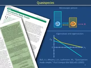
Quasispecies Microscopic picture A2 A1 X Eigenvalues and eigenvectors 0 Bull, J.J.; Meyers, L.A.; Lachmann, M.; “Quasispecies made simple,” PLoSComputBiol1(6):e61 (2005).
Microscopic perspective A2 A2 A2 A2 A2 A2 A2 A1 A1 A1 A1 A1 A1 A1 A1 Dt n1 n2
Microscopic perspective A2 A2 A2 A2 A2 A2 A2 A2 A2 A2 A2 A1 A1 A1 A1 A1 A1 A1 A1 A1 A1 A1 A1 A1 A1 Dt n1 n2
Microscopic perspective A2 A2 A2 A2 A2 A2 A2 A2 A2 A2 A2 A2 A2 A2 A2 A1 A1 A1 A1 A1 A1 A1 A1 A1 A1 A1 A1 A1 A1 Dt n1 n2
Microscopic perspective A2 A2 A2 A2 A2 A2 A2 A2 A2 A2 A2 A2 A2 A2 A1 A1 A1 A1 A1 A1 A1 A1 A1 A1 A1 A1 A1 A1 A1 Dt n1 n2
Microscopic perspective X A2 A2 A2 A2 A2 A2 A2 A2 A2 A2 A2 A2 A2 A1 A1 A1 A1 A1 A1 A1 A1 A1 A1 A1 A1 A1 A1 A1 Dt n1 n2
Microscopic perspective X X X A2 A2 A2 A2 A2 A2 A2 A2 A2 A2 A2 A2 A2 A2 A2 A2 A2 A2 A2 A2 A2 A2 A1 A1 A1 A1 A1 A1 A1 A1 A1 A1 A1 A1 A1 A1 A1 A1 A1 A1 A1 A1 X X Dt X n1 n2
Microscopic perspective X X X A2 A2 A2 A2 A2 A2 A2 A2 A2 A2 A2 A2 A2 A2 A2 A2 A2 A1 A1 A1 A1 A1 A1 A1 A1 A1 A1 A1 A1 A1 A1 A1 A1 A1 A1 A1 A1 X X Dt X n1 n2
Quasispecies Microscopic picture A2 A1 X Eigenvalues and eigenvectors 0 Bull, J.J.; Meyers, L.A.; Lachmann, M.; “Quasispecies made simple,” PLoSComputBiol1(6):e61 (2005).
Eigenvalues and eigenvectors Eigenvalues Eigenvectors
Eigenvalues and eigenvectors X A2 A1 Eigenvalues Eigendemographics 300 3 200 m1 = 2m2 m3 = 0.005 100 0 0.5 1.0 0 0.5 1.0 -100 -3 m2 -m3
Homework These graphs explore m2 > 0.5. This inappropriate. Why? What happens to the graphs of the eigenvalues and eigendemographics as m3 → 0? Can you use the equations derived in this slide deck to study the case m3 = 0? The ratio of the population of A2 cells to A1 cells in the eigenvector corresponding to l- is negative. For this eigenvector, the population of A2 cells will be negative if, for example, the population of A1 cells is positive. A negative cell population is non-physical. Nonetheless, we retain this eigenvector in order to analyze the dynamics of physical populations. Why? Read Bull, Meyers, and Lachmann’s green box. Distinguish an error catastrophe from an extinction catastrophe. X A2 A1 Eigenvalues Eigendemographics 300 3 200 m1 = 2m2 m3 = 0.005 100 0 0.5 1.0 0 0.5 1.0 -100 -3 m2 -m3