The Dark Side of Valuation. By Aswath Damodaran. New York University

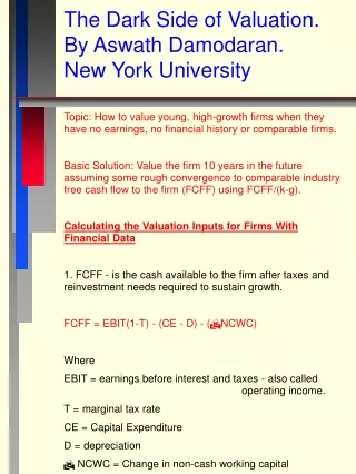
1. The Dark Side of Valuation. By Aswath Damodaran. New York University Topic: How to value young, high-growth firms when they have no earnings, no financial history or comparable firms. Basic Solution: Value the firm 10 years in the future assuming some rough convergence to comparable industry free cash flow to the firm (FCFF) using FCFF/(k-g). Calculating the Valuation Inputs for Firms With Financial Data 1. FCFF - is the cash available to the firm after taxes and reinvestment needs required to sustain growth. FCFF = EBIT(1-T) - (CE - D) - (NCWC) Where EBIT = earnings before interest and taxes - also called operating income. T = marginal tax rate CE = Capital Expenditure D = depreciation  NCWC = Change in non-cash working capital

2. 2. g = RR * ROC Where g = Expected Growth in EBIT RR = Reinvestment Rate = (CE - D + NCWC) ROC = Return on Capital = EBIT(1-T)/capital invested 3. Cost of capital = k = ke[E/(D+E)] + kd[D/(D+E)] Where ke = cost of equity kd = after-tax cost of debt E = market value of equity D = market value of debt 4. Terminal Valuen = FCFFn+1 / (kn - gn) This value is discounted back n years at the appropriate k that covers the first n years, usually 10 years. Although first ten years FCFF is estimated and discounted, value comes largely from value after 10 years for the young firms of interest here. All inputs should be sustainable rates.

3. 5. For the total firm value add the value of cash (C), marketable securities (MS) and other assets whose income is not consolidated in operating income (NOA). 6. Firm Value = C + MS + NOA + Note: We allow for different k in each of the first t years. 7. Equity Value = Firm Value - Debt Value 8. Equity Value Per Share = [Equity Value - Options Value]/ Shares Outstanding 9. Options values comes from management options, warrants and convertible debt or preferred.

4. Typical Methods to Handle Problems 1. Negative earnings - Use Normal Earnings A. past average over cycle - adjust for increase in scale if growth will occur in future B. Estimate normal operating or net profit margins or use prior years’ average or industry average and apply to revenue (which is never negative) C. Estimate normal ROC or use industry average and apply to invested capital. D. Reduce leverage over time - if negative earnings due to financing costs. Assume debt ratio goes to optimum (at lowest k) or use industry average. -assume firm reduces future investment to pay down debt, issues equity to pay down debt or grows to scale that can support current debt. 2. Note: In all cases if earnings are expected to normalize after some lag, not immediately, then estimate future normal earnings and discount back to present. Typically, the farther away current figures are from normal figures, the longer it is assumed to take until convergence to normal figures. If large growth is expected, then convergence may be quicker. 3. To handle tax effects of net operating losses (NOL), get PV of NOL = NOL(T)/(1+r)n where n is the year into which the losses are carried.

5. 4. When should normal earnings be used? - when losses are transient - or cyclical. - use profitability and current revenues or capital to estimate normal earnings when scale of firm is changing. - long-term operational/structural problems - require adjusting margins to sustainable levels - industry average of stable firms. If problems seem insurmountable - consider bankruptcy so no value (or perhaps option value).

6. Young Firms With No History or Apparent Comparable Industry Firms 1. Get data from firms as similar as possible even if not directly comparable. - Similar businesses - Amazon - retailers/booksellers. - Richness of information - more data on retailers than booksellers. - Life cycle similarity - data from retailers shows us how margins and revenue change with age. This can be used to project similar changes for a young firm - this is unavailable if we select an industry with only young firms. 2. Expected Revenue Growth alternatives - use most recent 12 months growth for firm - growth for market the firm serves - sustainability depends on barriers to entry or competitive advantages 3. Sustainable Operating Margin - examine true competitors - Amazon - Specialty retailers - adjust firms own negative margins by removing research, development and advertising that are unusually high but must be expensed rather than capitalized by GAAP.

7. 4. Reinvestment Needs - steady state - RR = g/ROC - all figures for steady state (see earlier) - assume RR growth = revenue growth - assume converges to RR = industry average RR A. Then get $reinvestment = RR*current $Capital B. Or use $reinvestment = $Revenues/ (S/C) where S/C = Revenues/ Capital 5. Risk - estimate beta from financial characteristics - use industry average (internet firms) or assume convergence to industry average (specialty retail) in future. 6. Estimate ke with CAPM and beta 7. Estimate kd with rate for bond rating - use 0 tax rate for loss period, carry-forward period and then apply full tax rate. 8. Use convergence to industry average capital structure D/(E+D). 9. Use compound cost of different yearly capital costs in later years which converge to stable rate for terminal value.

8. Final Value 1. Firm Value = C + MS + NOA + 2. Equity Value = Firm Value - Debt Value 3. Equity Value Per Share = [Equity Value - Options Value]/ Shares Outstanding 4. Perhaps adjust equity value for probability of default. Adjusted Equity Value Per Share = (Equity Value Per Share) * (1-default probability) 5. The most important value drivers are - sustainable margins - revenue growth - important but less - convergence time, reinvestment needs

9. Other Considerations 1. To deal with the uncertainty in pricing young firms - consider investing in a portfolio of those you find undervalued rather than the most undervalued -you could be mistaken on the one- I.e. diversify. 2. Valuation shows what type of assumptions are required to justify market price - assumptions may seem reasonable or not. 3. Earnings growth obtained by cutting investment below that required to remain competitive and sustain future earnings may be misleading. 4. Comparables methods are popular because they are often easier to apply but actually implicitly rely on the same assumptions as the FCFF method. The FCFF method makes the assumptions easier to see and judge for reasonability. For young firms, many get comparable ratio out 5-10 years and discount price back. Main problem: if all firms in comparable group are under or over-valued then results are bogus.