Download

1 / 6
100 likes | 417 Views
Inverse Heat Conduction Problem (IHCP) Applied to a High Pressure Gas Turbine Vane. David Wasserman MEAE 6630 Conduction Heat Transfer Prof. Ernesto Gutierrez-Miravete. Analyzing the entire geometry too difficult Simplify by analyzing as 1-Dimensional Transient Slab Problem

E N D
Inverse Heat Conduction Problem (IHCP) Applied to a High Pressure Gas Turbine Vane David Wasserman MEAE 6630 Conduction Heat Transfer Prof. Ernesto Gutierrez-Miravete
Analyzing the entire geometry too difficult • Simplify by analyzing as 1-Dimensional Transient Slab Problem • *non-homogeneous boundary conditions • *no heat generation • *no coatings
Problem: • Determine amount of heat flux necessary to keep vane below maximum operating temperature of superalloy to avoid microstructural damage • Boundary Conditions and Initial Condition: • Keep gaspath side fixed at maximum operating temperature, cool side subjected to heat flux • Assume cool side is initially at maximum operating temperature before cooling air is turned on (not true but simplified analysis) • Solution Method: • Assumed constant thermal properties obtained as the average of properties at maximum operating temperature and steady state temperature • Originally wanted to analyze as steady state problem but it was a limiting case and proved to be too complicated • Changed to transient analysis • -problem: did not have transient temperature measurements • -assume: cool side starts at maximum operating temperature and drops linearly to the steady state temperature
Inverse problems are ill-posed in that the solution does not satisfy requirements of • -existence • -uniqueness • -stability • Use minimization of least squares norm to guarantee existence of solution • After some computation and substitution we get the formal solution for IHCP • Alpha* - regularization parameter : helps with stability • X - matrix of sensitivity coefficients : change in temp wrt change in heat flux • Y - vector of measured temperatures from sensor at x = 0 surface • I - identity matrix • q - estimated heat flux at the surface
In order to calculate sensitivity coefficients, need to solve auxiliary problem • Nonhomogeneous auxiliary problem can be split into steady state problem and homogeneous problem Steady State Homogeneous B.C.’s Solution
Results and Conclusions: • Inverse problem solved using MATLAB program • Heat Flux is decreasing with time ---> might be correct trend • -Need large amount of flux at beginning, less at steady state • Steady state value obtained from program does not agree with steady state hand calc • Solved ex 5-3 to see if MATLAB program was correct--->Results were reassuring • Heat flux vector depends on method used to calculate temperature vector • Experiment with different “measured” temperature vectors • Substitute heat fluxes back into direct problem to get resulting temperatures as a check • Possibly try ANSYS