Asymmetric Information

Asymmetric Information

Asymmetric Information • Transactions can involve a considerable amount of uncertainty • can lead to inefficiency when one side has better information • The side with better information is said to have private information or asymmetric information

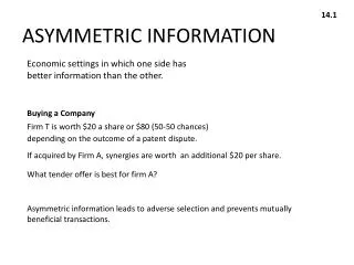
Asymmetric Information • Information cost may vary among agents as a result of differences in education and experience about commodity • Examples include • A firm possessing limited information about a potential worker’s abilities • A used car buyer not having complete repair and maintenance history on an auto • An insurance company not knowing risky behavior of a potential insurer

The Value of Contracts • Contractual provisions can be added in order to circumvent some of the inefficiencies associated with asymmetric information • Example: Insurance company can offer lower health insurance premium to customer who submit to medical exams • rarely do they eliminate them

Principal-Agent Model • The party who proposes the contract is called the principal • The party who decides whether or not to accept the contract and then performs under the terms of the contract is the agent • typically the party with asymmetric information

Leading Models • Two models of asymmetric information • the agent’s actions affect the principal, but the principal does not observe the actions directly • called a hidden-action model or a moral hazard model • the agent has private information before signing the contract (his type) • called a hidden-type model or an adverse selection model

First, Second, and Third Best • In a full-information environment, the principal could propose a contract that maximizes joint surplus • could capture all of the surplus for himself, leaving the agent just enough to make him indifferent between agreeing to the contract or not • This is called a first-best contract

First, Second, and Third Best • The contract that maximizes the principal’s surplus subject to the constraint that he is less well informed than the agent is called a second-best contract • Adding further constraints leads to the third best, fourth best, etc.

Hidden Actions • The principal would like the agent to take an action that maximizes their joint surplus • But, the agent’s actions may be unobservable to the principal • the agent will prefer to shirk • Contracts can mitigate shirking by tying compensation to observable outcomes

Hidden Actions • Often, the principal is more concerned with outcomes than actions anyway • may as well condition the contract on outcomes

Hidden Actions • The problem is that the outcome may depend in part on random factors outside of the agent’s control • tying the agent’s compensation to outcomes exposes the agent to risk • if the agent is risk averse, he may require the payment of a risk premium before he will accept the contract

Owner-Manager Relationship • Suppose a firm has one representative owner and one manager • the owner offers a contract to the manager • the manager decides whether to accept the contract and what action e 0 to take • an increase in e increases the firm’s gross profit but is personally costly to the manager (e – effort & time the manager puts in on the job)

Owner-Manager Relationship • The firm’s gross profit is g = e +  • where  represents demand, cost, and other economic factors outside of the agent’s control • assume  ~ (0,2) • c(e) is the manager’s personal disutility from effort / cost of undertaking effort • assume c’(e) > 0 and c’’(e) < 0

Owner-Manager Relationship • If s is the manager’s salary, the firm’s net profit is n = g– s • The risk-neutral owner wishes to maximize the expected value of profit E(n) = E(e +  –s) = e – E(s)

Owner-Manager Relationship • We will assume the manager is risk averse with a constant risk aversion parameter of A > 0 • The manager’s expected utility will be

First-Best (Full info case) • With full information, it is relatively easy to design an optimal salary contract • the owner can pay the manager a salary if he exerts a first-best level of effort and nothing otherwise • for the manager to accept the contract E(u) = s* - c(e*)  0

First-Best • The owner will pay the lowest salary possible [s* = c(e*)] • The owner’s net profit will be E(n) = e* - E(s*) = e* - c(e*) • at the optimum, the marginal cost of effort equals the marginal benefit

Second Best • If the owner cannot observe effort, the contract cannot be conditioned on e • the owner may still induce effort if some of the manager’s salary depends on gross profit • suppose the owner offers a salary such as s(g) = a + bg • a is the fixed salary and b is the power of the incentive scheme

Second Best • This relationship can be viewed as a three-stage game • owner sets the salary (choosing a and b) • the manager decides whether or not to accept the contract • the manager decides how much effort to put forth (conditional on accepting the contract)

Second Best • Because the owner cannot observe e directly and the manager is risk-averse, the second-best effort will be less than the first-best effort • the risk premium adds to the owner’s cost of inducing effort

First- versus Second-Best Effort The owner’s MC is higher in the second best, leading to lower effort by the manager MC in second best c’(e) + risk term MC in first best c’(e) MB 1 e e** e*

Moral Hazard in Insurance • If a person is fully insured, he will have a reduced incentive to undertake precautions • may increase the likelihood of a loss occurring

Moral Hazard in Insurance • The effect of insurance coverage on an individual’s precautions, which may change the likelihood or size of losses, is known as moral hazard

Mathematical Model • Suppose a risk-averse individual faces the possibility of a loss (l) that will reduce his initial wealth (W0) • the probability of loss is  • an individual can reduce this probability by spending more on preventive measures (e)

Mathematical Model • An insurance company offers a contract involving a payment of x to the individual if a loss occurs • the premium is p • If the individual takes the coverage, his expected utility is E[u(W)] = (1-)u(W0-e-p) + ()u(W0-e-p-l+x)

First-Best Insurance Contract • In the first-best case, the insurance company can perfectly monitor e • should set the terms to maximize its expected profit subject to the participation constraint • the expected utility with insurance must be at least as large as the utility without the insurance • will result in full insurance with x = l • the individual will choose the socially efficient level of precaution

Second-Best Insurance Contract • Assume the insurance company cannot monitor e at all • an incentive compatibility constraint must be added • The second-best contract will typically not involve full insurance • exposing the individual to some risk induces him to take some precaution

Hidden Types • In the hidden-type model, the individual has private information about an innate characteristic he cannot choose • the agent’s private information at the time of signing the contract puts him in a better position

Hidden Types • The principal will try to extract as much surplus as possible from agents through clever contract design • include options targeted to every agent type

Nonlinear Pricing • Consider a monopolist who sells to a consumer with private information about his own valuation for the good • The monopolist offers a nonlinear price schedule • menu of different-sized bundles at different prices • larger bundles sell for lower per-unit price

Mathematical Model • Suppose a single consumer obtains surplus from consuming a bundle of q units for which he pays a total tariff of T u = v(q) – T • assume that v’(q) > 0 and v’’(q) < 0 • the consumer’s type is  • H is the “high” type (with probability of ) • L is the “low” type (with probability of 1-) • 0 < L < H

Mathematical Model • Suppose the monopolist has a constant average and marginal cost of c • The monopolist’s profit from selling q units is  = T – cq

First-Best Nonlinear Pricing • In the first-best case, the monopolist observes  • At the optimum v’(q) = c • the marginal social benefit of increased quantity is equal to the marginal social cost

First-Best Nonlinear Pricing This graph shows the consumers’ indifference curves (by type) and the firm’s isoprofit curves T U0H U0L q

First-Best Nonlinear Pricing A is the first-best contract offered to the “high” type and B is the first-best offer to the “low” type T U0H A U0L B q

Second-Best Nonlinear Pricing • Suppose the monopolist cannot observe  • knows the distribution • Choosing A is no longer incentive compatible for the high type • the monopolist must reduce the high-type’s tariff

To keep him from choosing B, the monopolist must reduce the “high” type’s tariff by offering a point like C C Second-Best Nonlinear Pricing The “high” type can reach a higher indifference curve by choosing B T U0H A U2H U0L B q

Second-Best Nonlinear Pricing The monopolist can also alter the “low” type’s bundle to make it less attractive to the high type T U0H A E U2H C U0L B D q q**H q**L

Monopoly Coffee Shop • The college has a single coffee shop • faces a marginal cost of 5 cents per ounce • The representative customer faces an equal probability of being one of two types • a coffee hound (H = 20) • a regular Joe (L = 15) • Assume v(q) = 2q0.5

First Best • Substituting such that marginal cost = marginal benefit, we get q = (/c)2 q*L = 9 q*H = 16 T*L = 90 T*H = 160 E() = 62.5

Incentive Compatibility when Types Are Hidden • The first-best pricing scheme is not incentive compatible if the monopolist cannot observe type • keeping the cup sizes the same, the price for the large cup would have to be reduced by 30 cents • the shop’s expected profit falls to 47.5

Second Best • The shop can do better by reducing the size of the small cup • The size that is second best would be LqL-0.5 = c + (H - L)qL-0.5 q**L = 4 T**L = 60 E() = 50

Adverse Selection in Insurance • Adverse selection is a problem facing insurers where the risky types are more likely to accept an insurance policy and are more expensive to serve • assume policy holders may be one of two types • H = high risk • L = low risk

First Best • The insurer can observe the individual’s risk type • First best involves full insurance • different premiums are charged to each type to extract all surplus

First Best W2 U0L Without insurance each type finds himself at E certainty line U0H B A and B represent full insurance A E W1

Second Best • If the insurer cannot observe type, first-best contracts will not be incentive compatible • if the insurer offered A and B, the high-risk type would choose B • the insurer must change the coverage offered to low-risk individuals to make it unattractive to high-risk individuals

The high-risk type is fully insured, but his premium is higher (than it would be at B) C D The low-risk type is only partially insured First Best W2 U0L U1H certainty line U0H B A E W1

Market Signaling • If the informed player moves first, he can “signal” his type to the other party • the low-risk individual would benefit from providing his type to insurers • he should be willing to pay the difference between his equilibrium and his first-best surplus to issue such a signal

Market for Lemons • Sellers of used cars have more information on the condition of the car • but the act of offering the car for sale can serve as a signal of car quality • it must be below some threshold that would have induced the owner to keep it

Market for Lemons • Suppose there is a continuum of qualities from low-quality lemons to high-quality gems • only the owner knows a car’s type • Because buyers cannot determine the quality, all used cars sell for the same price • function of average car quality

Asymmetric Information