Download
1 / 39
410 likes | 731 Views
Chapter 8. AVL Search Trees. [INA240] Data Structures and Practice Youn-Hee Han http://link.kut.ac.kr. 1. AVL Tree Basic Concepts. Motivation Complexity of BST Average case: O(log n) Inserting sorted data Worst case: O(n) If BST is unbalanced, the efficiency is bad. Balance ( 복습 )

E N D
Chapter 8. AVL Search Trees [INA240] Data Structures and Practice Youn-Hee Han http://link.kut.ac.kr
1. AVL Tree Basic Concepts • Motivation • Complexity of BST • Average case: O(log n) • Inserting sorted data • Worst case: O(n) • If BST is unbalanced, the efficiency is bad. • Balance (복습) • : the height of the left subtree • : the height of the right subtree • Balance factor (B) = HL – HR • Balanced binary tree: |B| 1 HL HR Data Structure
1. AVL Tree Basic Concepts • AVL Tree: a binary search tree in which the heights of the subtrees differ by no more than 1 • |HL-HR|<=1 for all nodes • HL-HR is called balance factor • An AVL is a balanced tree • Invented by G.M Adelson-Velskii and E.M. Landis, 1962. Data Structure
1. AVL Tree Basic Concepts • AVL Tree Example (교재 Fig. 8-2, pp. 343) LH: left high (+1) EH: even high(0) RH: eight high(-1) Data Structure
-1 10 1 1 7 40 0 0 1 -1 3 8 30 45 0 0 0 -1 0 1 5 20 35 60 0 25 1. AVL Tree Basic Concepts • Is It an AVL Tree? • Is It an AVL Tree? Data Structure
1. AVL Tree Basic Concepts • AVL Trees • Non-AVL Trees Data Structure
1. AVL Tree Basic Concepts • AVL 트리에서노드의 선언 • 삽입과 삭제시 고려졈 • Balance Factor의 범위가 넘어선 노드 확인 • 삽입, 삭제가 일어나면 반드시 해당 위치로부터 루트까지 올라가면서 모든 노드에 대한 Balance Factor가 그 범위를 넘어섰는지 확인 typedef struct node { void* dataPtr; 데이터 필드 struct node* left; 왼쪽 자식을 가리키는 포인터 struct node* eight; 오른쪽 자식을 가리키는 포인터 int bal; Balance Factor } NODE; 노드는 구조체 타입 Disadvantage: needs extra storage for maintaining node balance Data Structure
2. Balancing Tree - Insert • Inserting a node into an AVL tree 1. Connect the new node to a leaf node with the same algorithm with BST insertion 2. Check the balance of each node for all ancestor nodes of the new node 3. If an unbalanced node “r” is found, rebalance it and then continue up the tree • Not all insertion breaks the balance Data Structure
3 5 2 5 3 6 4 6 1 4 2 1 Node 4 attached to new parent 2. Balancing Tree - Insert • Rotation: switching children and parents among two or three adjacent nodes to restore balance of a tree. • Rotation with Re-attachment Data Structure
-2 0 -1 Mar Mar Mar -1 0 May May 0 0 Nov rotation May 0 0 Mar Nov 2. Balancing Tree - Insert • A rotation may change the depth of some nodes, but does not change their relative ordering. • Insertion-> unbalancing -> rebalancing Data Structure
2. Balancing Tree - Insert • All unbalanced tree fall into one of these 4 cases - for the nearest unbalanced ancestor r from the new node n • Left of left: A subtree (r) that is left high has also become left high r n n Case I-1: left of left (complex) r n n Case I-2: left of left (simple) Data Structure
2. Balancing Tree - Insert • All unbalanced tree fall into one of these 4 cases • for the nearest unbalanced ancestor r from the new node n • Right of right: A subtree (r) that is right high has also become right high r n n Case II-1: right of right (complex) r n n Case II-2: right of right (simple) Data Structure
2. Balancing Tree - Insert • All unbalanced tree fall into one of these 4 cases - for the nearest unbalanced ancestor r from the new node n • Right of left: A subtree (r) that is left high has included right high subtree r n Case III-1: right of left (complex) r n n Case III-2: right of left (simple) Data Structure
2. Balancing Tree - Insert • All unbalanced tree fall into one of these 4 cases • for the nearest unbalanced ancestor r from the new node n • Left of right: A subtree (r) that is right high has included left high subtree r n Case IV-1: left of right (complex) r n n Case IV-2: left of right (simple) Data Structure
2. Balancing Tree - Insert • Case I: Left of left 경우 “LL Rotation” 으로 해결 • 불균형 노드 r의 왼쪽 서브트리의 왼쪽 서브트리에 새 노드 Y가 삽입된 경우 • 마지막의 RChild에 삽입되는 경우와, LChild에 삽입되는 경우 BF: 2 BF: 2 12 12 L L L 7 L 7 20 20 3 10 3 10 5 2 Data Structure
2. Balancing Tree - Insert • LL Rotation 원리 – Single Right Rotation After rotation, BF(x) = 0, BF(r) = 0,-1,1 * r: nearest ancestor of the new node whose BF(r) is +2 or -2 Data Structure
2. Balancing Tree - Insert • LL Rotation Examples Data Structure
2. Balancing Tree - Insert • Case II: Right of Right 경우 “RR Rotation” 으로 해결 • 불균형 노드 r의 오른쪽 서브트리의 오른쪽 서브트리에 새 노드 Y가 삽입된 경우 • RR Rotation 원리 – Single Left Rotation After rotation, BF(x) = 0, BF(r) = 0,-1,1 Data Structure
2. Balancing Tree - Insert • RR Rotation Examples Data Structure
2. Balancing Tree - Insert • Case III: Right of Left 경우 “LR Rotation” 으로 해결 • 불균형 노드 r의 왼쪽 서브트리의 오른쪽 서브트리에 새 노드 Y가 삽입된 경우 • LR Rotation 원리 – Double Rotation After rotation, BF(x) = 0, BF(r) = 0,-1,1 Data Structure
2. Balancing Tree - Insert • LR Rotation Examples Data Structure
2. Balancing Tree - Insert • LR Rotation Examples Data Structure
2. Balancing Tree - Insert • Case IV: Left of Right 경우 “RL Rotation” 으로 해결 • 불균형 노드 r의 오른쪽 서브트리의 왼쪽 서브트리에 새 노드 Y가 삽입된 경우 • RL Rotation 원리 – Double Rotation After rotation, BF(x) = 0, BF(r) = 0,-1,1 Data Structure
2. Balancing Tree - Insert • RL Rotation Examples Data Structure
3. Balancing Tree - Delete • Deleting a node into an AVL tree 1. Deleting the node with the same algorithm with BST deletion 2. Check the balance of each node for all ancestor nodes of the altered and lowest node 3. If an unbalanced node “r” is found, rebalance it and then continue up the tree • Not all insertion breaks the balance Data Structure
3. Balancing Tree - Delete • For example r BF: 2 Case I - left of left deleting LL rotation Data Structure
3. Balancing Tree - Delete • For example r BF: 2 Case I - left of left deleting LL rotation Data Structure
3. Balancing Tree - Delete • For example r BF: -2 deleting 35 Case I - left of left 41 41 42 42 LL rotation 41 35 41 (c) Data Structure
4. Efficiency of AVL Trees • AVL 트리 • 가장 먼저 시도된 균형 트리 이론 • 균형을 잡기 위해 트리 모습을 수정 • 실제 코딩면에서 볼 때 AVL 트리는 매우 까다롭고 복잡 • 트리의 균형 • 탐색효율 O(lgN)을 보장 • 삽입, 삭제 될 때마다 균형 파괴여부 검사하는 시간이 필요 • 트리를 재구성(Rebuilding)하는 시간이 필요 • 통계적으로 삽입, 삭제 이후… • 회전이 필요없는 경우: 54% • LL/RR 회전이 필요한 경우: 23% • LR/RL 회전이 필요한 경우: 23% Data Structure
5. 스플레이(Splay) 트리 • 일반적인 균형 트리 (Balanced Tree)의 특징 • 균형트리는 최악의 경우에라도 무조건 lgN 시간에 탐색하기 위함 • 루트로부터 리프까지 가는 경로를 최소화하기 위함 • 하지만, 모든 노드가 동일한 빈도(Frequency)로 탐색되는 것은 아님 • 자체 조정 트리 (Self-Restructuring Tree) – Splay Tree • Sleator and Tarjan (1985) • (Original Paper: http://www.cs.cmu.edu/~sleator/papers/self-adjusting.pdf) • 탐색의 빈도를 기준으로 스스로 트리 모습을 재 구성하는 트리 • 무조건 균형을 유지할 것이 아니라 자주 탐색되는 노드를 루트 근처에 갖다 놓는 것이 더욱 유리 Tree Binary Tree AVL Search Tree Binary Search Tree A splay tree is a self-balancing binary search tree (BST) with the additional unusual property that recently accessed elements are quick to access again. – [wikipedia] Splay Tree Data Structure
5. 스플레이(Splay) 트리 • 조정방법 I • 어떤 노드가 탐색될 때마다 그 노드를 바로 위 부모 노드로 올리는 방법 • 한번의 회전만으로 충분함. 예: 키 3인 노드 탐색결과 • 탐색될 때 마다 부모로 올라가므로 탐색 빈도가 높은 노드들은 점차 루트 주위로 모인다. Data Structure
5. 스플레이(Splay) 트리 • 조정방법 II • 어떤 노드가 탐색되면 그 노드를 전체 트리의 루트로 옮김 • 한번 탐색된 노드는 이후에 탐색될 가능성이 높다고 간주 • 연속적인 회전이 필요 • 예: 노드 3의 탐색결과. • 회전시마다 자식노드의 오른쪽 서브트리는 부모노드의 왼쪽 서브트리로 연결됨 Data Structure
5. 스플레이(Splay) 트리 • 조정방법 II의 단점 • 트리의 균형 면에서 불리 • 노드 1의 탐색결과. 트리의 높이는 줄지 않고, 그대로 유지됨 Data Structure
5. 스플레이(Splay) 트리 • 스플레이(Splay, 바깥으로 펼치는 (보기흉한…)) • 조정방법 II를 개선 • 탐색된 노드를 루트로 올리되, 한번에 두 레벨씩 위로 올림. • 다음의 세가지 스플레이 스텝연산이 존재함 • Zig-Zag step • Zig-Zig step • Zig step Data Structure
5. 스플레이(Splay) 트리 • Zig-Zig step • 두 번의 step • 1st 올림: 탐색된 노드의 부모 노드를 기준으로 올림 • 2nd올림: 탐색된 노드 자체를 기준으로 올림 • AVL에서 LL 또는 RR 회전 원리와 비슷하지 않음 (^^) • 예] 키 3인 노드를 탐색. 루트에서 키 3까지는 Zig-Zig. Single Rotation Data Structure
5. 스플레이(Splay) 트리 • Zig-Zag step • AVL의 LR 또는 RL회전과 완전 동일 • Zig-Zag step 예 Double Rotation Data Structure
5. 스플레이(Splay) 트리 • Zig step • AVL에서 단순한 경우의 LL 회전및 RR 회전과 동일 Data Structure
5. 스플레이(Splay) 트리 • 스플레이에 의한 균형 • LChild, RChild 링크가 벌어지기 (Splay) 때문에 어느 정도 균형이 맞추어짐 • 하지만, Balance Factor가 -1, 0, 1로 유지되어야 하는 것은 아님 • 스플레이 트리 • 트리의 균형보다는 노드 자체의 탐색빈도를 더 우선시 하는 트리 • 어떤 노드가 상대적으로 다른 노드보다 자주 사용된다면 유리한 구조 • 모두 동일한 빈도로 사용된다면 Splay의 장점은 없음 Zig-Zig Zig Zig-Zig Data Structure
[참고] 이진트리의 순회법 • Inorder (중위) Traversal • Preorder (전위) Traversal • Postorder (후위) Traversal • Traversal 순서 알아내는 좋은 방법 Data Structure