Download
1 / 21
210 likes | 372 Views
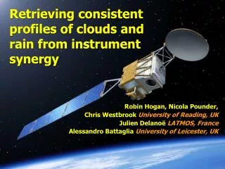
Retrieving consistent profiles of clouds and rain from instrument synergy. Robin Hogan, Nicola Pounder University of Reading, UK Julien Delanoë LATMOS, France. Overview.

E N D
Retrieving consistent profiles of clouds and rain from instrument synergy Robin Hogan, Nicola Pounder University of Reading, UK Julien Delanoë LATMOS, France
Overview • The synergy of instruments in the A-Train and EarthCARE offer more accurate retrievals of cloud & light precipitation than ever before • But to exploit integral measurements (radar PIA, radiances) we must retrieve cloud and precipitation simultaneously • Variational approach offers rigorous treatment of errors • Behaviour should tend towards existing two-instrument synergy algos • Radar+lidar for ice clouds: Donovan et al. (2001), Delanoe & H (2008) • DARDAR available at: http://www.icare.univ-lille1.fr/projects/dardar/ • CloudSat+MODIS for liquid clouds: Austin & Stephens (2001) • Calipso+MODIS for aerosol: Kaufman et al. (2003) • CloudSat surface return for rainfall: L’Ecuyer & Stephens (2002) • This talk presents progress towards “unified algorithm” for EarthCARE • Retrieval framework • Automatic adjoints • Ice, rain and melting-ice retrieval: testing on simulated profiles • Demonstration on A-Train data • Future work
Unified retrieval Ingredients developed Implement previous work Not yet developed 1. New ray of data: define state vector Use classification to specify variables describing each species at each gate Ice: extinction coefficient, N0’,lidar extinction-to-backscatter ratio Liquid: extinction coefficient and number concentration Rain: rain rate, drop diameter and melting ice Aerosol: extinction coefficient, particle size and lidar ratio 2. Convert state vector to radar-lidar resolution Often the state vector will contain a low resolution description of the profile 3. Forward model 6. Iteration method Derive new state vector using quasi-Newton scheme 3a. Radar model Including surface return and multiple scattering 3b. Lidar model Including HSRL channels and multiple scattering 3c. Radiance model Solar and IR channels Not converged 4. Compare to observations Check for convergence Converged 7. Calculate retrieval error Error covariances and averaging kernel Proceed to next ray of data
Unified retrieval: forward model • From state vector x to forward modelled observations H(x)... Gradient of cost function (vector) xJ=HTR-1[y–H(x)] x Ice & snow Liquid cloud Rain Aerosol Lookup tables to obtain profiles of extinction, scattering & backscatter coefficients, asymmetry factor Ice/radar Ice/lidar Ice/radiometer Liquid/radar Liquid/lidar Liquid/radiometer Vector-matrix multiplications: around the same cost as the original forward operations Rain/radar Rain/lidar Rain/radiometer Aerosol/radiometer Aerosol/lidar Sum the contributions from each constituent Lidar scattering profile Radar scattering profile Radiometer scattering profile Adjoint of radiometer model Adjoint of radar model (vector) Adjoint of lidar model (vector) Radiative transfer models H(x) Adjoint of radiative transfer models Lidar forward modelled obs Radar forward modelled obs Radiometer fwd modelled obs yJ=R-1[y–H(x)]
Minimization methods - in 1D • Gauss-Newton method • Requires the curvature 2J/x2 • A matrix • More expensive to calculate • Fewer iterations to converge • Assume J is quadratic and jump to the minimum • Limited to smaller retrieval problems 2J/x2 J J/x J/x x1 x1 x2 x3 x2 x4 x3 x5 x6 x4 x7 x8 x5 x Quasi-Newton method (e.g. L-BFGS) • Rolling a ball down a hill • Smart choice of direction in many dimensions aids convergence • Requires the gradient J/x • A vector (efficient to store) • Efficient to calculate using adjoint method • Used in data assimilation J x Coding up adjoints and Jacobian matrices is very time consuming and error prone – is there a better way?
Automatic adjoints • Quite fiddly and error-prone to code-up dJ/dx given dJ/dy • Algorithm y(x) in C++: • adouble algorithm(const adouble x[2]) { • adouble y = 4.0; • adouble s = 2.0*x[0] + 3.0*x[1]*x[1]; • y *= sin(s); • return y; • } • // Main code • adept::Stack stack; • y = algorithm(x); • stack.compute_adjoint(); // Do the hard work • double algorithm_AD(const double x[2], • double y_AD[1], double x_AD[2]) { • double y = 4.0; • double s = 2.0*x[0] + 3.0*x[1]*x[1]; • y *= sin(s); • /* Adjoint part: */ • double s_AD = 0.0; • y_AD[0] += sin(s) * y_AD[0]; • s_AD += y * cos(s) * y_AD[0]; • x_AD[0] += 3.0 * s_AD; • x_AD[1] += 6.0 * x[0] * s_AD; • s_AD = 0.0; • y_AD[0] = 0.0; • return y; • } • double algorithm(const double x[2]) { • double y = 4.0; • double s = 2.0*x[0] + 3.0*x[1]*x[1]; • y *= sin(s); • return y; • } • This can be done automatically in C++ using a special active type “adouble” and overloading mathematical operators and functions • Existing libraries CppAD and ADOL-C provide this capability but they’re quite slow • New library “Adept” uses expression templates in C++ to do this much faster • Freely available at http://www.met.rdg.ac.uk/clouds/adept • Hogan (Mathematics & Computers in Simulation, in review)
Tested PVC and TDTS multiple scattering algorithms (here for PVC) Time relative to original code for profile with N=50 cloudy points: Adjoint calculation is: Only 5-20% slower than hand-coded adjoint 5-9 times faster than leading alternative libraries ADOL-C and CppAD Jacobian calculation is: 4-20 times faster than ADOL-C/CppAD for a matrix of size 50x350 Now used for entire unified algorithm Sorry, it won’t work for Fortran until Fortran has template capability! Benchmark results
Retrieved (state) variables Ice clouds and snow (extension of Delanoe and Hogan 2008, 2010) [1] log extinction coefficient, [2] log lidar ratio [3] log number conc parameter N0* (good a priori from temperature) [4] “Riming factor” to allow Doppler information to be assimilated Lidar molecular signal is used beyond cloud, when detectable Liquid clouds (see Nicola Pounder’s talk) [1] log LWC, [2] total number concentration (one value per liquid layer) Extinction info from lidar multiple scattering, radar PIA, SW radiances Rain and melting ice [1] log rain rate, [2] number conc parameter Nw* (one value per profile) “Flatness constraint” on rain rate: extra terms in cost function penalize deviations from a constant rain rate with height Different a-priori values for stratocu drizzle and rain from melting ice Melting layer radar attenuation uses Matrosov’s empirical relationship: 2-way attenuation [dB] = 2.2 x rain rate [mm h-1] Additional term in cost function penalizes difference in snow flux above melting layer and rain rate below Use radar PIA information over the ocean
Idealized nimbostratus retrieval Constraint of constant flux across melting layer and smooth rain profile, but we have the classic ill-constrained attenuation retrieval problem
Idealized nimbostratus retrieval Much better behaviour with flatness constraint on rain rate
A-Train case • Forward modelled radar and lidar match observations well, indicating good convergence • Can also simulate the Doppler velocity that would be observed by EarthCARE • Currently omits multiple scattering and air motion effects on Doppler
Retrievals • Ice cloud properties retrieved similarly to Delanoe and Hogan (2008, 2010) algorithm • Water flux is approximately conserved across the melting layer • Rain rate is relatively constant with range
Forward models and observations Implement LIDORT solar radiance model (has adjoint/Jacobian) Implement Delanoe & Hogan infrared radiance code Implement multiple scattering model with depolarization (but are measurements too noisy?) Incorporate radar path integrated attenuation Incorporate Doppler velocity Retrieved quantities Add “riming” factor Refine aerosol retrieval Verification Consistency of different sources of information using A-Train data Aircraft data with in-situ sampling from NASA ER-2 and French aircraft EarthCARE simulator (ECSIM) scenes using EarthCARE specification Further work
Minimizing the cost function Gradient of cost function (a vector) Gauss-Newton method Rapid convergence (instant for linear problems) Get solution error covariance “for free” at the end Levenberg-Marquardt is a small modification to ensure convergence Need the Jacobian matrix H of every forward model: can be expensive for larger problems as forward model may need to be rerun with each element of the state vector perturbed • and 2nd derivative (the Hessian matrix): • Gradient Descent methods • Fast adjoint method to calculate xJ means don’t need to calculate Jacobian • Disadvantage: more iterations needed since we don’t know curvature of J(x) • Quasi-Newton method to get the search direction (e.g. L-BFGS used by ECMWF): builds up an approximate inverse Hessian A for improved convergence • Scales well for large x • Poorer estimate of the error at the end
Ice fall speeds Terminal fall-speed (m s-1) • Heymsfield & Westbrook (2010) expression predicts fall speed as a function of particle mass, maximum dimension and “area ratio” • Currently we assume Brown and Francis (1995) mass-size relationship, so fall speed is a function of size alone Brown & Francis (1995) • In convective clouds, intend to add a multiplication factor (or similar) to allow denser particles (e.g. rimed aggregates, graupel and hail) to be retrieved using the Doppler measurements
Simple melting-layer model • Minimalist approach: • 2-way radar attenuation in dB is 2.2 times rain rate (Matrosov 2008) • No effect on other variables • Add term to cost function penalizing difference between ice flux above and rain flux below melting layer Matrosov (IEEE Trans. Geosci. Rem. Sens. 2008)
A mixed-phase case Observations • Retrievals
Use “DARDAR” CloudSat-CALIPSO cloud mask How well is mean cloud fraction modelled? Tend to underestimate mid & low cloud fraction How good are models at forecasting cloud at right time? (SEDI skill score) Winter mid to upper troposphere: excellent Tropical mid to upper troposphere: fair Tropical and sub-tropical boundary layer: virtually no skill! Hogan, Stein, Garcon & Delanoe (in prep) Model skill