Download
1 / 33
330 likes | 490 Views
Hidden Markov Models Reading: Russell and Norvig , Chapter 15, Sections 15.1-15.3. Recall for Bayesian networks: General question: Given query variable X and observed evidence variable values e , what is P ( X| e )? . Dynamic Bayesian Networks.

E N D
Hidden Markov ModelsReading: Russell and Norvig, Chapter 15, Sections 15.1-15.3
Recall for Bayesian networks: General question: Given query variable X and observed evidence variable values e, what is P(X|e)?
Dynamic Bayesian Networks • General dynamic Bayesian network: any number of random variables, which can be discrete or continuous • Observations are taken in time steps. • At each time step, observe some of the variables (evidence variables). Other variables are unobservedor “hidden”.
Simple example of HMM(adapted from Russell and Norvig, Chapter 15) You are a graduate student in a windowless office with no phone and your network connection is down. The only way you can get information about the weather outside is whether or not your advisor shows up carrying an umbrella.
P(Rain0 =T ) = 0.5 HMM for this scenario: Evidence variable: Umbrella {T, F} Hidden variable Rain {T, F} Markov model since Rt depends only on Rt-1. Raint-1 Raint Raint+1 Umbrellat-1 Umbrellat Umbrellat+1
Inference in Hidden Markov Models • Inference tasks: • Filtering (or monitoring): Computing belief state―posterior distribution over current state, given all evidence to date: “Given that my advisor has had an umbrella for the last three days, what’s the probability it is raining today?”
Inference in Hidden Markov Models • Prediction: Computing posterior distribution over the future state, given all evidence to date: “Given that my advisor has had an umbrella for the last three days, what’s the probability it will rain the day after tomorrow?”
Smoothing (or hindsight): Computing posterior probability over a past state, given all evidence up to the present: “Given that my advisor has had an umbrella for the last three days, what’s the probability it rained yesterday?
Most likely explanation: Given a sequence of observations, finding the sequence of states most likely to have generated those observations: “Given that my advisor has had an umbrella for the last three days, what’s the most likely sequence of weather over the past 3 days?”
Inference algorithms • Filtering: Can use recursive estimation
Inference algorithms • Filtering: Can use recursive estimation The value of the first term, , is given explicitly in the network.
Inference algorithms • Filtering: Can use recursive estimation The value of the first term, , is given explicitly in the network. The value of the second term is:
Inference algorithms • Filtering: Can use recursive estimation The value of the first term, , is given explicitly in the network. The value of the second term is: Thus:
Inference algorithms From the network, we have everything except P(xt, e1:t). Can estimate recursively. Thus:
Umbrella example: • Day 1: Umbrella1 = U1 = T Prediction t = 0 to t = 1: Updating with evidence for t=1:
Prediction t = 1 to t = 2: Updating with evidence for t=2: Why does probability of rain increase from day 1 to day 2?
Hidden Markov Models: Matrix Representations • Transition model: P(Xt| Xt1) = T (SS matrix) where • For umbrella model: • Sensor model: P(et | Xt = i ) =O (SS diagonal matrix) where • For umbrella model:
Speech Recognition • Task: Identify sequence of words uttered by speaker, given acoustic signal. • Uncertainty introduced by noise, speaker error, variation in pronunciation, homonyms, etc. • Thus speech recognition is viewed as problem of probabilistic inference.
Speech recognition typically makes three assumptions: • Process underlying change is itself “stationary” i.e., state transition probabilities don’t change • Current state X depends on only a finite history of previous states (“Markov assumption”). • Markov process of order n: Current state depends only on n previous states. • Values et of evidence variables depend only on current state Xt. (“Sensor model”)
Speech Recognition • Input: acoustic signal • Inference: P(words | signal) • Bayes rule: P(words | signal) = P(signal | words) P(words) • P(signal | words): acoustic model • pronunciation model (for each word, distribution over possible phone sequences) • signal model (distribution of features of acoustic signal over phones) • P(words): language model – prior probability of each utterance (e.g., bigram model)
Russell and Norvig, Artificial Intelligence: A Modern Approach, Chapter 15
Phone model P( phone | frame features) = P(frame features| phone) P(phone) P(frame features| phone) often represented by Gaussian mixture model
Pronunciation model Now we want P (words|phones1:t ) = P(phones1:t | words) P(words) Represent P(phones1:t | words) as an HMM
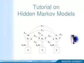
More Generally: Components of an HMM P(Rain0 =T ) = 0.5 Raint-1 Raint Raint+1 Umbrellat-1 Umbrellat Umbrellat+1 Model consists of sequence of hidden states, sequence of observation states, probability of each hidden state given previous hidden state, probability of each hidden state given current observation, and prior probability of first hidden state.
Possible states: S = {S1, ..., SN} P(Rain0 =T ) = 0.5 Raint-1 Raint Raint+1 Umbrellat-1 Umbrellat Umbrellat+1 Model consists of sequence of hidden states, sequence of observation states, probability of each hidden state given previous hidden state, probability of each hidden state given current observation, and prior probability of first hidden state.
State transition probabilities A = [aij], aij=P(qt+1=Sj|qt=Si) P(Rain0 =T ) = 0.5 Raint-1 Raint Raint+1 Umbrellat-1 Umbrellat Umbrellat+1 Model consists of sequence of hidden states, sequence of observation states, probability of each hidden state given previous hidden state, probability of each hidden state given current observation, and prior probability of first hidden state.
P(Rain0 =T ) = 0.5 Possible observations (or “emissions”): V={v1, ..., vM} Raint-1 Raint Raint+1 Umbrellat-1 Umbrellat Umbrellat+1 Model consists of sequence of hidden states, sequence of observation states, probability of each hidden state given previous hidden state, probability of each hidden state given current observation, and prior probability of first hidden state.
Observation (emission) probabilities: B = [bj(m)] bj(m)=P(Ot=vm|qt=Si) P(Rain0 =T ) = 0.5 Raint-1 Raint Raint+1 Umbrellat-1 Umbrellat Umbrellat+1 Model consists of sequence of hidden states, sequence of observation states, probability of each hidden state given previous hidden state, probability of each hidden state given current observation, and prior probability of first hidden state.
Initial state probabilities: = [i] i =P(q1=Si) P(Rain0 =T ) = 0.5 Raint-1 Raint Raint+1 Umbrellat-1 Umbrellat Umbrellat+1 Model consists of sequence of hidden states, sequence of observation states, probability of each hidden state given previous hidden state, probability of each hidden state given current observation, and prior probability of first hidden state.
Learning an HMM Baum-Welch algorithm (also known as “forward-backward algorithm), similar to Expectation-Maximization