Speech & Audio Processing
Speech & Audio Processing. Speech & Audio Coding Examples. A Simple Speech Coder. LPC Based Analysis Structure. Linear Prediction Analysis. Levinson- Durbin. Pre- emphasis. Windowing Analysis. Auto- Correlation. Audio Input. Residual. Residual. Analysis Filter. Quantization.

Speech & Audio Processing
E N D
Presentation Transcript
Speech & Audio Processing Speech & Audio Coding Examples
A Simple Speech Coder • LPC Based Analysis Structure Linear Prediction Analysis Levinson-Durbin Pre-emphasis WindowingAnalysis Auto-Correlation AudioInput Residual Residual AnalysisFilter Quantization Filter Coeffs Filter Coeffs Veton Këpuska
Windowing Analysis Stage N – Length of the Analysis Window 10-30 msec Veton Këpuska
Some Analysis Windows Veton Këpuska
MATLAB Useful Functions • wintool • Use “doc wintool” for more information • window • Use “>doc window” for the list of supported windows • Define your own window if needed e.g: • Sine window and Vorbis window Veton Këpuska
LPC Analysis Stage • LPC Method Described in: • Ch5-Analysis_&_Synthesis_of_Pole-Zero_Speech_Models.ppt • Summary: • Perform Autocorrelation • Solve system of equations with Durbin-Levinson Method • MATLAB help • doc lpc, etc. Veton Këpuska
Example of MATLAB Code function myLPCCodec(wavfile, N) % % wavfile - input MS wav file % N - LPC Filter Order % [x, fs, nbits] = wavread(wavfile); % plot(x); % Playing Original Signal soundsc(x,fs); % Performing LPC analysis using MATLAB lpc function [a, g] = lpc(x,N); % performing filtering operation on estimated filter coeffs % producing predicted samples est_x = filter([0 -a(2:end)], 1, x); % error signal e = x - est_x; % Testing the quality of predicted samples soundsc(est_x, fs); % Synthesis Stage With Zero Loss of Information syn_x = filter([0 -a(2:end)], 1, g.*e); soundsc(syn_x,fs); ŝ[n] ge[n] Veton Këpuska
Analysis of Quantization Errors • Use MATLAB functions to research the effects of quantization errors introduced by precision of the arithmetic operations and representation of the filter and error signal: • Double (float64) representation (software emulation) • Float (float32) representation (software emulation) • Int (int32) representation (hardware emulation) • Short (int16) representation (hardware emulation). • Useful MATLAB functions: • Fix, floor, round, ceil • Example: • sig_hat=fix(sig*2^(B-1))/2^(B-1); • Truncation of the sig to B bits. Veton Këpuska
Quantization of Error Signal & Filter Coefficients • Can Apply ADPCM for Error Signal • Filter Coefficients in the Direct Filter Form are found to be sensitive to quantization errors: • Small quantization error can have a large effect on filter characteristics. • Issue is that polynomial coefficients have non-linear mapping to poles of the filter (e.g., roots of the polynomial). • Alternate representations possible that have significantly better tolerance to quantization error. Veton Këpuska
LPC Filter Representations • As noted previously when Levinson-Durbin algorithm was introduced one alternate representation to filter coefficients was also mentioned: PARCOR coefficients: • LPC to PARCOR: Veton Këpuska
PARCOR Filter Representation • PARCOR to LPC: Veton Këpuska
Line Spectral Frequency Representation • It turns out that PARCOR coefficients can be represented with LSF that have significantly better properties. • Note that: • The PARCOR lattice structure of the LPC synthesis filter above: Input Output Ap-1 A0 Ap + + kp kp-1 k0=-1 kp+1=∓1 - - z-1 z-1 z-1 Bp-1 B0 Bp Veton Këpuska
Line Spectral Frequency Representation • From previous slide the following holds: • From this realization of the filter the LSP representation is derived: Veton Këpuska
LSF Representation Veton Këpuska
LPC Synthesis Filter with LSF Veton Këpuska
A Simple Speech Coder • LPC Based Synthesis Structure ResidualSignal De-emphasis SynthesisFilter AudioOutput Residual Decoding Filter Coeffs FilterCoeffs Veton Këpuska
Audio Coding • Most of the Audio Coding Standards use principles of Psychoacoustics. • Example of Basic Structure of MP3 encoder: AudioInput Bit-stream Filterbank &Transform Quantization PsychoacousticModel Veton Këpuska
Basic Structure of Audio Coders • Filterbank Processing • Psychoacoustic Model • Quantization Veton Këpuska
Filterbank Processing: • Splitting full-band signal into several sub-bands: • Uniform sub-bands (FFT) • Critical Band (FFT followed by non-linear transformation) • Reflect Human Auditory Apparatus. • Mel-Scale and Bark-Scale transformations Veton Këpuska
Mel-Scale Veton Këpuska
Bark-Scale Veton Këpuska
Analysis Structure of Filterbank hk[n] – Impulse Response of a Quadrature Mirror kth-filter N – Number of Channels. Typically 32 ↓ - Down-sampling MDCT – Modified Discrete Cosine Transform h1[n] ↓ MDCT MDCT Bit Stream AudioInput hk[n] ↓ MDCT MDCT Quantization hN[n] ↓ MDCT MDCT Veton Këpuska
Analysis Structure of Filterbank gk[n] – Impulse Response of a Inverse Quadrature Mirror kth-filter N – Number of Channels. Typically 32 ↑ - Up-sampling IMDCT – Inverse Modified Discrete Cosine Transform IMDCT ↑ g1[n] MDCT Bit Stream AudioOutput IMDCT ↑ gk[n] MDCT Decoding IMDCT ↑ gN[n] MDCT Veton Këpuska
Psychoacoustic Model • Masking Threshold according to the human auditory perception. • Masking threshold is used to quantize the Discrete Cosine Transform Coefficients • Analysis is done in frequency domain represented by DFT and computed by FFT. Veton Këpuska
Threshold of Hearing • Absolute threshold of audibly perceptible events in quiet conditions (no other sounds). • Any signal bellow the threshold can be removed without effect on the perception. Veton Këpuska
Threshold of Hearing Veton Këpuska
Frequency Masking • Schröder Spreading Function • Bark Scale Function: Veton Këpuska
Masking Curve Veton Këpuska
Primary Tone 1kHz Veton Këpuska
Masked Tone 900 Hz Veton Këpuska
Combined Sound 1kHz + 0.9kHz Veton Këpuska
Combined 1kHz + 0.9kHz (-10dB) Veton Këpuska
Combined 1kHz + 5kHz (-10dB) Veton Këpuska
END Veton Këpuska