Bayesian models of inductive learning

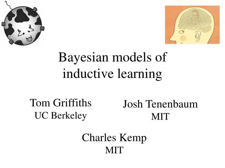
Bayesian models of inductive learning Tom Griffiths UC Berkeley Josh Tenenbaum MIT Charles Kemp MIT

What to expect • What you’ll get out of this tutorial: • Our view of what Bayesian models have to offer cognitive science. • In-depth examples of basic and advanced models: how the math works & what it buys you. • Some (not extensive) comparison to other approaches. • Opportunities to ask questions. • What you won’t get: • Detailed, hands-on how-to. • Where you can learn more: • http://bayesiancognition.com • Trends in Cognitive Sciences, July 2006, special issue on “Probabilistic Models of Cognition”.

Outline • Morning • Introduction: Why Bayes? (Josh) • Basic of Bayesian inference (Josh) • Graphical models, causal inference and learning (Tom) • Afternoon • Hierarchical Bayesian models, property induction, and learning domain structures (Charles) • Methods of approximate learning and inference, probabilistic models of semantic memory (Tom)

Why Bayes? • The problem of induction • How does the mind form inferences, generalizations, models or theories about the world from impoverished data? • Induction is ubiquitous in cognition • Vision (+ audition, touch, or other perceptual modalities) • Language (understanding, production) • Concepts (semantic knowledge, “common sense”) • Causal learning and reasoning • Decision-making and action (production, understanding) • Bayes gives a general framework for explaining how induction can work in principle, and perhaps, how it does work in the mind….

P(grammar | UG) P(phrase structure | grammar) P(utterance | phrase structure) P(speech | utterance) (c.f. Chater and Manning, 2006) “Universal Grammar” Hierarchical phrase structure grammars (e.g., CFG, HPSG, TAG) Grammar Phrase structure Utterance Speech signal

The approach • Key concepts • Inference in probabilistic generative models • Hierarchical probabilistic models, with inference at all levels of abstraction • Structured knowledge representations: graphs, grammars, predicate logic, schemas, theories • Flexible structures, with complexity constrained by Bayesian Occam’s razor • Approximate methods of learning and inference: Expectation-Maximization (EM), Markov chain Monte Carlo (MCMC) • Much recent progress! • Computational resources to implement and test models that we could dream up but not realistically imagine working with • New theoretical tools let us develop models that we could not clearly conceive of before.

Vision as probabilistic parsing (Han and Zhu, 2006)

“tufa” “tufa” “tufa” Word learning on planet Gazoob Can you pick out the tufas?

Learning word meanings Whole-object principle Shape bias Taxonomic principle Contrast principle Basic-level bias Principles Structure Data

Causal learning and reasoning Principles Structure Data

Goal-directed action (production and comprehension) (Wolpert et al., 2003)

Marr’s Three Levels of Analysis • Computation: “What is the goal of the computation, why is it appropriate, and what is the logic of the strategy by which it can be carried out?” • Algorithm: Cognitive psychology • Implementation: Neurobiology

Alternative approaches to inductive learning and inference • Associative learning • Connectionist networks • Similarity to examples • Toolkit of simple heuristics • Constraint satisfaction • Analogical mapping

Summary: Why Bayes? • A unifying framework for explaining cognition. • How people can learn so much from such limited data. • Strong quantitative models with minimal ad hoc assumptions. • Why algorithmic-level models work the way they do. • A framework for understanding how structured knowledge and statistical inference interact. • How structured knowledge guides statistical inference, and may itself be acquired through statistical means. • What forms knowledge takes, at multiple levels of abstraction. • What knowledge must be innate, and what can be learned. • How flexible knowledge structures may grow as required by the data, with complexity controlled by Occam’s razor.

Outline • Morning • Introduction: Why Bayes? (Josh) • Basic of Bayesian inference (Josh) • Graphical models, causal inference and learning (Tom) • Afternoon • Hierarchical Bayesian models, property induction, and learning domain structures (Charles) • Methods of approximate learning and inference, probabilistic models of semantic memory (Tom)

Likelihood Prior probability Posterior probability Bayes’ rule For any hypothesis h and data d, Sum over space of alternative hypotheses

Bayesian inference • Bayes’ rule: • An example • Data: John is coughing • Some hypotheses: • John has a cold • John has emphysema • John has a stomach flu • Prior favors 1 and 3 over 2 • Likelihood P(d|h) favors 1 and 2 over 3 • Posterior P(d|h) favors 1 over 2 and 3

Coin flipping • Basic Bayes • data = HHTHT or HHHHH • compare two simple hypotheses: P(H) = 0.5 vs. P(H) = 1.0 • Parameter estimation (Model fitting) • compare many hypotheses in a parameterized family P(H) = q : Infer q • Model selection • compare qualitatively different hypotheses, often varying in complexity: P(H) = 0.5 vs. P(H) = q

Coin flipping HHTHT HHHHH What process produced these sequences?

Comparing two simple hypotheses • Contrast simple hypotheses: • h1: “fair coin”, P(H) = 0.5 • h2:“always heads”, P(H) = 1.0 • Bayes’ rule: • With two hypotheses, use odds form

Comparing two simple hypotheses D: HHTHT H1, H2: “fair coin”, “always heads” P(D|H1) = 1/25P(H1) = ? P(D|H2) = 0 P(H2) = 1-?

Comparing two simple hypotheses D: HHTHT H1, H2: “fair coin”, “always heads” P(D|H1) = 1/25P(H1) = 999/1000 P(D|H2) = 0 P(H2) = 1/1000

Comparing two simple hypotheses D: HHHHH H1, H2: “fair coin”, “always heads” P(D|H1) = 1/25 P(H1) = 999/1000 P(D|H2) = 1 P(H2) = 1/1000

Comparing two simple hypotheses D: HHHHHHHHHH H1, H2: “fair coin”, “always heads” P(D|H1) = 1/210 P(H1) = 999/1000 P(D|H2) = 1P(H2) = 1/1000

The role of intuitive theories The fact that HHTHT looks representative of a fair coin and HHHHH does not reflects our implicit theories of how the world works. • Easy to imagine how a trick all-heads coin could work: high prior probability. • Hard to imagine how a trick “HHTHT” coin could work: low prior probability.

Coin flipping • Basic Bayes • data = HHTHT or HHHHH • compare two hypotheses: P(H) = 0.5 vs. P(H) = 1.0 • Parameter estimation (Model fitting) • compare many hypotheses in a parameterized family P(H) = q : Infer q • Model selection • compare qualitatively different hypotheses, often varying in complexity: P(H) = 0.5 vs. P(H) = q

Parameter estimation • Assume data are generated from a parameterized model: • What is the value of q ? • each value of q is a hypothesis H • requires inference over infinitely many hypotheses q d1d2 d3 d4 P(H) = q

s1 s2 s3 s4 Model selection • Assume hypothesis space of possible models: • Which model generated the data? • requires summing out hidden variables • requires some form of Occam’s razor to trade off complexity with fit to the data. q d1 d2 d3 d4 d1 d2 d3 d4 d1 d2 d3 d4 Hidden Markov model: si {Fair coin, Trick coin} Fair coin: P(H) = 0.5 P(H) = q

Parameter estimation vs. Model selection across learning and development • Causality: learning the strength of a relation vs. learning the existence and form of a relation • Language acquisition: learning a speaker's accent, or frequencies of different words vs. learning a new tense or syntactic rule (or learning a new language, or the existence of different languages) • Concepts: learning what horses look like vs. learning that there is a new species (or learning that there are species) • Intuitive physics: learning the mass of an object vs. learning about gravity or angular momentum • Intuitive psychology: learning a person’s beliefs or goals vs. learning that there can be false beliefs, or that visual access is valuable for establishing true beliefs

Parameter estimation: A hierarchical learning framework model parameters data

Model selection: Parameter estimation: A hierarchical learning framework model class model parameters data

Bayesian parameter estimation • Assume data are generated from a model: • What is the value of q ? • each value of q is a hypothesis H • requires inference over infinitely many hypotheses q d1d2 d3 d4 P(H) = q

Some intuitions • D = 10 flips, with 5 heads and 5 tails. • q = P(H) on next flip? 50% • Why? 50% = 5 / (5+5) = 5/10. • Why? “The future will be like the past” • Suppose we had seen 4 heads and 6 tails. • P(H) on next flip? Closer to 50% than to 40%. • Why? Prior knowledge.

Integrating prior knowledge and data • Posterior distribution P(q| D)is a probability density over q = P(H) • Need to work out likelihood P(D | q ) and specify prior distribution P(q )

Likelihood and prior • Likelihood: Bernoulli distribution P(D | q ) = q NH(1-q ) NT • NH: number of heads • NT: number of tails • Prior: P(q )  ?

Some intuitions • D = 10 flips, with 5 heads and 5 tails. • q = P(H) on next flip? 50% • Why? 50% = 5 / (5+5) = 5/10. • Why? Maximum likelihood: • Suppose we had seen 4 heads and 6 tails. • P(H) on next flip? Closer to 50% than to 40%. • Why? Prior knowledge.

A simple method of specifying priors • Imagine some fictitious trials, reflecting a set of previous experiences • strategy often used with neural networks or building invariance into machine vision. • e.g., F ={1000 heads, 1000 tails} ~ strong expectation that any new coin will be fair • In fact, this is a sensible statistical idea...

Likelihood and prior • Likelihood: Bernoulli(q ) distribution P(D | q ) = q NH(1-q ) NT • NH: number of heads • NT: number of tails • Prior: Beta(FH,FT)distribution P(q ) q FH-1 (1-q ) FT-1 • FH: fictitious observations of heads • FT: fictitious observations of tails

Shape of the Beta prior

Shape of the Beta prior FH = 0.5, FT = 0.5 FH = 0.5, FT = 2 FH = 2, FT = 0.5 FH = 2, FT = 2

Bayesian parameter estimation • Posterior is Beta(NH+FH,NT+FT) • same form as prior! • expected P(H) = (NH+FH) / (NH+FH+NT+FT) P(q | D)  P(D | q ) P(q ) = q NH+FH-1(1-q ) NT+FT-1

Conjugate priors • A prior p(q ) is conjugate to a likelihood function p(D | q ) if the posterior has the same functional form of the prior. • Parameter values in the prior can be thought of as a summary of “fictitious observations”. • Different parameter values in the prior and posterior reflect the impact of observed data. • Conjugate priors exist for many standard models (e.g., all exponential family models)

Some examples • e.g., F ={1000 heads, 1000 tails} ~ strong expectation that any new coin will be fair • After seeing 4 heads, 6 tails, P(H) on next flip = 1004 / (1004+1006) = 49.95% • e.g., F ={3 heads, 3 tails} ~ weak expectation that any new coin will be fair • After seeing 4 heads, 6 tails, P(H) on next flip = 7 / (7+9) = 43.75% Prior knowledge too weak

But… flipping thumbtacks • e.g., F ={4 heads, 3 tails} ~ weak expectation that tacks are slightly biased towards heads • After seeing 2 heads, 0 tails, P(H) on next flip = 6 / (6+3) = 67% • Some prior knowledge is always necessary to avoid jumping to hasty conclusions... • Suppose F = { }: After seeing 1 heads, 0 tails, P(H) on next flip = 1 / (1+0) = 100%

Origin of prior knowledge • Tempting answer: prior experience • Suppose you have previously seen 2000 coin flips: 1000 heads, 1000 tails

Problems with simple empiricism • Haven’t really seen 2000 coin flips, or any flips of a thumbtack • Prior knowledge is stronger than raw experience justifies • Haven’t seen exactly equal number of heads and tails • Prior knowledge is smoother than raw experience justifies • Should be a difference between observing 2000 flips of a single coin versus observing 10 flips each for 200 coins, or 1 flip each for 2000 coins • Prior knowledge is more structured than raw experience

A simple theory • “Coins are manufactured by a standardized procedure that is effective but not perfect, and symmetric with respect to heads and tails. Tacks are asymmetric, and manufactured to less exacting standards.” • Justifies generalizing from previous coins to the present coin. • Justifies smoother and stronger prior than raw experience alone. • Explains why seeing 10 flips each for 200 coins is more valuable than seeing 2000 flips of one coin.

A hierarchical Bayesian model physical knowledge Coins • Qualitative physical knowledge (symmetry) can influence estimates of continuous parameters (FH, FT). q~ Beta(FH,FT) FH,FT ... Coin 1 Coin 2 Coin 200 q200 q1 q2 d1d2 d3 d4 d1d2 d3 d4 d1d2 d3 d4 • Explains why 10 flips of 200 coins are better than 2000 flips of a single coin: more informative about FH, FT.

Bayesian models of inductive learning